Ozone Transport to the San Joaquin Valley

Uncontrollable sources of ozone from stratospheric intrusions, wildfires, and intercontinental transport are complicating efforts in California to further reduce this pollutant, which is particularly harmful to our health.

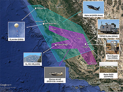
Scientists measured daily fluctuations in ozone in the air across Northern and Central California in 2016 during a coordinated field campaign known as the California Baseline Ozone Transport Study. They particularly focused on ozone crossing the shoreline and accumulating in low level air over the San Joaquin Valley.

Ian Faloona (University of California, Davis) and colleagues summarize the measurements and unique meteorological context for this novel dataset in a recent article published in the Bulletin of the American Meteorological Society. Faloona et al. draw attention to the dataset’s potential for future modeling studies of the impacts of long-range transport on regional air quality.

FaloonaIaninCockpit

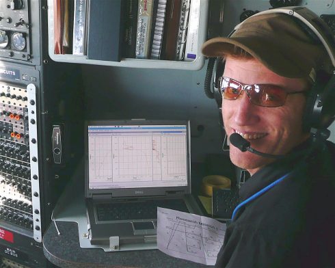
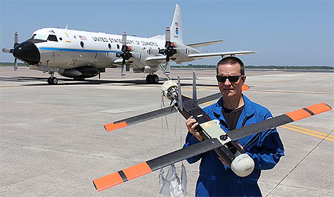
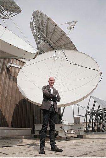
Falloona, in his cockpit perch during aerial measurements for CABOTS.

We asked lead author Faloona to help us understand CABOTS and his motivations for this work.

BAMS: What would you like readers to learn from this article?

Faloona: I think this article presents a nice overview of the mesoscale flow over the complex terrain of Central and Northern California, and I would like readers to become more appreciative of the global nature of air pollution. The field of air quality was once considered in terms of emissions and receptors within “air basins” but as our knowledge of the global nature of greenhouse gases in terms of climate change has developed, I believe that we have similarly become more and more aware of the global aspects of many air pollutants in general.

The CABOTS study domain and measurement platforms ranged from daily ozonesondes launched at the two coastal sites (Bodega Bay and Half Moon Bay) to the NOAA TOPAZ lidar in Visalia. The green and purple polygons represent the approximate domains surveyed by the NASA Alpha jet and Scientific Aviation, Inc., Mooney air-craft, respectively.


How did you become interested in the topic of this article?

Some colleagues from the UC Davis Air Quality Research Center and I became interested in long-range transport of air pollution to California and how it might be best sampled along the coastal mountains where local emissions might be minimal and the surface was well above the strong temperature inversion of the marine boundary layer. We eventually found the site on Chews Ridge where a group of renegade astronomers had been operating an off-the-grid observatory with the Monterey Institute for Research in Astronomy. They allowed us to build a climate monitoring site collocated with their observatory (the Oliver Observing Station) and then some airborne work for the San Joaquin Valley Air Pollution Control District allowed us to link the inflow at the coast to air quality issues within the leeward valley.

What got you initially interested in meteorology or in the related field you are in?

While an undergraduate studying physical chemistry I wrote a term paper on acid rain for a chemical oceanography class. I was floored by how few details were thoroughly understood about the chemical mechanisms of an environmental problem that at the time was considered quite serious. I figured I should throw whatever brainpower heft I could into this type of atmospheric oxidation chemistry.  But then, while working for a private consulting company in Colorado after college, many of my colleagues there were trained in meteorology and I knew there would be little progress without a fundamental understanding that field.  So I went to Penn State to do chemistry research but get trained in all aspects of meteorology.

What surprises/surprised you the most about the work you document in this article?

The first thing that surprised me about the data we collected for CABOTS was how deep the daytime up-valley flow was (~1.5 km), but how shallow the convective boundary layers tended to be (~0.5 km).  The scale interactions that need to be taken into account when analyzing boundary layers among the complex terrain of California make it a great place to study in meteorology. But the other major discovery that came out of this work was the evidence we found of significant NOx emissions from certain agricultural regions in the San Joaquin Valley. For instance, we found that the agricultural region between Fresno and Visalia was responsible for as much NOx emitted to the valley atmosphere as from all the mobile sources in the CARB inventory across the three county region.

What was the biggest challenge you encountered while doing this work?

The sensible heat at the Fresno airport.  Our airborne deployments attempted to target high ozone episodes, which are best forecast by their correlation with ambient temperatures. I like to tell my students that I am a chaser of extreme weather. It just so happens that the weather features most important to air quality are heat waves. Heat waves are extremely easy to catch, and can be brutal in their persistence.  Some days we observed temperatures in the plane on the tarmac of >115 ºF, which made it challenging to keep the equipment up and running. I remember dragging bags of ice in and out of the plane covered in sweat, and still having the instruments give up in heat exhaustion before one of our midday flights.

What’s next? How will you follow up?

I would like to continue studying the various scales at play in the transport of intercontinental pollution to North America, and my preferred tools are aircraft laboratories. I would like to follow up with a study of wintertime stagnation events that lead to particulate matter air quality problems – an entirely different meteorological beast.  But I would also like to follow up with a study of agricultural NOx emissions in the Imperial Valley of Southern California. This region is expected to have the largest soil emissions and the lowest urban sources to confound the measurements. It is also a region of important environmental justice issues being made up largely of migrant agricultural workers who have to bear the burden of the air quality problems engendered by agriculture.


Intuitive Metric for Deadly Tropical Cyclone Rains

With hurricanes moving more slowly and climate models projecting increasing rain rates, scientists have been grappling with how to effectively convey the resulting danger of extreme rains from these more intense, slow-moving storms.

C_Bosma
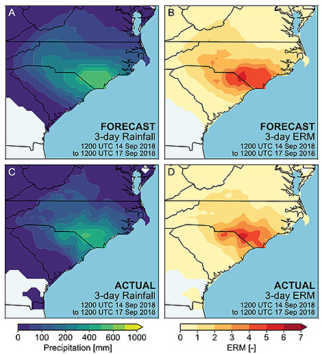
Flooding rainfall already is the most deadly hazard from tropical cyclones (TCs), which include hurricanes and tropical storms. Yet the widely recognized tool for conveying potential tropical cyclone destruction is the Saffir-Simpson Scale, which is based only on peak wind impacts. It categorizes hurricanes from 1, with winds causing minimal damage, to 5 and catastrophic wind damage. But it is unreliable for rain.

Recent research by Christopher Bosma, with the University of Wisconsin in Madison, and colleagues published in the Bulletin of the American Meteorological Society introduces a new tool that focuses exclusively on the deadly hazard of extreme rainfall in tropical cyclones. “Messaging the deadly water-related threat in hurricanes was a problem brought to light with Hurricanes Harvey and Florence,” says J. Marshall Shepherd (University of Georgia), one of the coauthors. “Our paper is offering a new approach to this critical topic using sound science methods.”

“One goal of this paper,” Bosma explains, “is to give various stakeholders—from meteorologists to emergency planners to the media—an easy-to-understand, but statistically meaningful way of talking about the frequency and magnitude of extreme rainfall events.”

That way is with their extreme rainfall multiplier (ERM), which frames the magnitude of rare extreme event rainfalls as multiples of baseline “heavy” rainstorms. Scientifically, ERM is the ratio of a specific location’s storm rainfall and the maximum amount of rain that has fallen most often at the location in two consecutive-year periods from 1981 through 2010—the baseline rain events that are relatively frequent at that location. A recurring baseline heavy rain amount is defined by the median (rather than the mean) annual maximum rainfall during the 30-year period and is used to weed out outlier events.

The authors are proposing the scale to

1. Accurately characterize the TC rainfall hazard;

2. Identify “locally extreme” events because local impacts increase with positive deviations from the local rainfall climatology;

3. Succinctly describe TC rainfall hazards at a range of time scales up to the lifetime of the storm system;

4. Be easy to understand and rooted in experiential processing to effectively communicate the hazard to the public.

Experiential processing is a term meaning rooted in experience, and ERM aims to relate its values for an extreme rainfall event to someone’s direct experience, or media reports and images, of heavy rainfall at their location. Doing this has the benefit of enabling them to connect, or “anchor” in cognitive psychology terms, the sheer magnitude of an extreme rain event to the area’s typical heavy rain events, highlighting how much worse it is.

Highest annual maximum ERMs (1948–2017) are indicated with colored markers and colored lines representing linear regression fit. A Mann–Kendall test for monotonic trends in annual maxima values did not reveal significant changes over time for either ERM or rainfall.


The researchers analyzed 385 hurricanes and tropical storms that either struck or passed within 500 km of land from 1948 through 2012 and, through hindcasting, determined an average ERM of 2.0. Nineteen of the storms had ERMs greater than 4.0. And disastrous rain-making hurricanes in the record had ERMs directly calculated as benchmark storms. These include the most extreme event, Hurricane Harvey with an ERM of 6.4, Hurricane Florence as well as 1999’s Hurricane Floyd, which swamped the East Coast from North Carolina to New England, (ERMs: 5.7), and Hurricane Diane (ERM: 4.9), which destroyed large swaths of the Northeast United States with widespread flooding rains in 1955, ushering “in a building boom of flood control dams throughout New England,” says, coauthor Daniel Wright, Bosma’s advisor at UW-Madison.

Wright says that a major challenge in developing ERM was maintaining scientific accuracy while widening its use to non-meteorologists.

I’ve been reading and writing research papers for more than 10 years that were written for science and engineering audiences. This work was a little different because, while we wanted the science to be airtight, we needed to aim for a broader audience and needed to “keep it simple.”

In practice, these historical values of ERM would be used to convey the severity of the rainfall hazard from a landfalling storm. For example the authors successfully hindcast ERM values  in the Carolinas for Hurricane Florence, which inundated southeastern portions of North Carolina and northeastern South Carolina as it crawled ashore in 2018. With an active tropical storm or hurricane, the forecast value of ERM could be compared with historical hurricanes that have hit the expected landfall location.

Verification of the National Weather Service forecasts for the 3-day rainfall after landfall of Hurricane Florence (and ERM forecasts derived from these QPF estimates), issued at 1200 UTC 14 Sep 2018. Actual rainfall and 3-day ERM are based on poststorm CPC-Unified data.

Verification of NWS forecasts for the 3-day rainfall after landfall of Hurricane Florence (and ERM forecasts derived from these QPF estimates), issued at 1200 UTC 14 Sep 2018. Actual rainfall and 3-day ERM are based on poststorm CPC-Unified data.


In theory, the sound science is such that the ERM framework could be applied to other rain-producing storms.

“We think there is potential both for characterizing the spatial properties of all kinds of extreme rainstorms…and then also for examining how these properties are changing over time,” Wright says.

The researchers caution, however, that there are things that must be resolved before ERM can be used operationally as a communication tool. For example, ERM will need to be scaled to be compatible with NWS gridded rainfall products and generalized precipitation forecasts.  Forecast lead times and event durations also will need to be determined. And graphical displays and wording still need to be worked out to communicate ERM most effectively.

Nevertheless, the team argues:

…our Hurricane Florence ERM hindcast shows that the method can accurately characterize the rainfall hazard of a significant TC several days ahead in a way that can be readily communicated to, and interpreted by, the public.

D_Wright

Above, Daniel Wright, of the University of Wisconsin-Madison

Active Hurricane Seasons: Maybe For 2020, But Not Necessarily in a Warmer Future

For a fifth consecutive year, NOAA is forecasting an above-average number of tropical cyclones (TCs) in the Atlantic, with 13-19 named storms expected in 2020. The number of TCs includes both tropical storms and hurricanes. This is in line with recent hurricane season forecasts by The Weather Channel, Penn State, Tropical Storm Risk, and others.

NOAA-2020-outlook

The recent spate of highly-active TC seasons, however, contrasts sharply with future trends in a majority of climate models, which simulate decreasing annual numbers of TCs as Earth’s climate continues to warm. That’s one of a number of findings in a recent paper by Tom Knutson (NOAA) and colleagues in the Bulletin of the American Meteorological Society.

In the paper, a team of tropical meteorology and hurricane experts led by Knutson assessed model projections of TCs in a world 2°C warmer than pre-industrial levels. The authors indicated mixed confidence in a downward TC frequency trend, even though 22 of 27 climate models the authors reviewed indicating the decrease. Some reputable models, though a minority, showed the frequency in named storms will instead increase in a warmer world, which lowered confidence in this particular finding.

As noted in Knutson et al. (2019, Part I of their two-part study: “Tropical Cyclones and Climate Change Assessment”), there is no clear observational evidence for a detectable human influence on historical global TC frequency. Therefore, there is no clear observational evidence to either support or refute the notion of decreased global TC frequency with climate warming. This apparent discrepancy between model projections and historical observations could be due to a number of factors. Among these are the relatively short available global TC records, the relatively modest expected sensitivity of global TC frequency to global warming since the 1970s, errors arising from limitations of model projections, differences between historical climate forcings and those used for twenty-first-century projections, or even observational limitations. However, the growing TC observational databases may soon provide a means of distinguishing between some highly divergent modeled scenarios of global TC frequency.

An average hurricane season in the Atlantic, which includes storms forming in the Caribbean Sea and Gulf of Mexico, sees 12 named storms with 6 becoming hurricanes. Of those hurricanes, typically three strengthen their sustained winds above 110 mph, becoming major hurricanes.

NOAA’s forecast cited warmer-than-usual sea surface temperatures, light winds aloft, and the lack of an El Niño, which tends to shear apart hurricanes, as factors for this year’s potentially active season. “Similar conditions have been producing more active seasons since the current high-activity era began in 1995,” NOAA stated in a release Thursday.

Knutson and his colleagues explain that the reason or reasons for a future decrease in TC frequency is uncertain, even as a warmer world would mean a continuation of warming seas. One possibility, the team entertains, is a decrease in large-scale rising air, termed “upward mass flux,” in the future. Its mechanism, however, is unclear, they find. Another is a reduction in saturation of the middle atmosphere in the models. Both are unfavorable for TC genesis.

The authors state that projections of TC frequency in different TC basins are “less robust” than the global signal. Comparing basins, they did find that the southwest Pacific and southern Indian oceans had greater TC decreases than the Atlantic and the Eastern and Western Pacific oceans.

They conclude this portion of the study stating that “reconciling projection results with theories or mechanistic understanding of TC genesis may eventually lead to improved confidence in projections of TC frequency.”

Knutson’s team found greater certainty in other facets of future TCs in the same study. For example, they expressed medium-to-high confidence that hurricanes will become stronger and wetter by the end of the twenty-first century.

New Assessment Is Confident Global Warming Brings Stronger, Wetter Tropical Cyclones

Even with a modest amount of global warming, future hurricanes will become nastier. They’ll push ashore higher storm surges, grow into superstorms like Hurricanes Dorian and Irma more often, and unleash inundating rains similar to Hurricanes Harvey and Florence more frequently.

That’s the assessment of published, peer-reviewed research in the past decade, according to an assessment by Thomas Knutson (NOAA) and colleagues, recently published in the Bulletin of the American Meteorological Society. It’s the second in a two part study conducted by the author team, 11 experts in climate and tropical cyclones (TCs). Part 1 found there are indeed already detectable changes in tropical cyclone activity attributable to human-caused climate change. Part 2, in the March 2020 BAMS online, project changes in the climatology of these storms worldwide due to human-induced global warming of just 2°C.

Highest confidence among the experts was in storm surge flooding. Rising sea levels due to warming and expanding oceans, responding to atmospheric warming and glacial ice melt, are already making it easier for hurricanes and even tropical storms to drive greater amounts of seawater ashore at landfall. And this will only worsen.

With CO2 levels climbing to about 414 ppm in March, as measured atop Mauna Loa in Hawaii, Earth is on track to reach a 2°C average global temperature increase by mid century. Already global average surface temperature has risen 1.2°C since the Industrial Revolution began.

In the assessment the authors have medium-to-high-confidence that rainfall rates in tropical cyclones will increase globally by 14% due to the increasing amount of water vapor available in a warmer atmosphere. They project a 5% global increase in tropical cyclone intensity along with an increase in the number of Category 4 and 5s ̶ although the range of opinions among the experts involved is 1-10%. In the Atlantic Basin, which includes the Caribbean Sea and Gulf of Mexico, the number of storms is projected to decrease while intensity as well as the number of intense hurricanes increases.

Other studies found that hurricanes will slow down, making them even more prolific rainmakers, among other changes. Authors of the new assessment discussed these additional changes, but cited less confidence in general and that different tropical basins around the world had different projections:

Author opinion was more mixed and confidence levels generally lower for some other TC projections, including a further poleward expansion of the latitude of maximum intensity of TCs in the western North Pacific basin, a decrease of global TC frequency, and an increase in the global frequency (as opposed to proportion) of very intense (category 4–5) TCs. The vast majority of modeling studies project decreasing global TC frequency (median of about −13% for 2°C of global warming), while a few studies project an increase. It is difficult to identify/quantify a robust consensus in projected changes in TC tracks across studies, although several project either poleward or eastward expansion of TC occurrence over the North Pacific. Projected TC size metric changes are on the order of 10% or less, and highly variable between basins and studies. Confidence in projections of TC translation speed is low due to the potential for data artifacts in the observed slowdown and a lack of model consensus. Confidence in various TC projections in general was lower at the individual basin scale than for the global average.

 Summary of TC projections for a 2°C global anthropogenic warming. Shown for each basin and the globe are median and percentile ranges for projected percentage changes in TC frequency, category 4–5 TC frequency, TC intensity, and TC near-storm rain rate. For TC frequency, the 5th–95th-percentile range across published estimates is shown. For category 4–5, TC frequency, TC intensity, and TC near-storm rain rates the 10th–90th-percentile range is shown. Note the different vertical-axis scales for the combined TC frequency and category 4–5 frequency plot vs the combined TC intensity and TC rain rate plot. See the supplemental material for further details on underlying studies used.
Summary of TC projections for a 2°C global anthropogenic warming. Shown for each basin and the globe are median and percentile ranges for projected percentage changes in TC frequency, category 4–5 TC frequency, TC intensity, and TC near-storm rain rate. For TC frequency, the 5th–95th-percentile range across published estimates is shown. For category 4–5, TC frequency, TC intensity, and TC near-storm rain rates the 10th–90th-percentile range is shown.

Website Tracks Public Understanding of Tornadoes

Imagine you live in a part of the country where few people have experienced tornadoes. It would make sense that your neighbors wouldn’t know the difference between a tornado watch or warning, or know how to seek safety.

A new, openly available online tool shows exactly that, by combining societal databases with survey results about people’s understanding of weather information. But there are some surprising wrinkles in the data. For example, the database drills down to county-level information and finds “noteworthy differences” within regions of similar tornado climatology.

How is it that Norman, Oklahoma, residents score higher in what people think they know of severe weather information than those in Fort Worth, Texas? And why is there a similar gap between what people actually do know, as tested in Peachtree City, Georgia, versus Birmingham, Alabama?

“Differences like this create important opportunities for research and learning within the weather enterprise,” say Joseph T. Ripberger and colleagues, who describe the weather demographics tool in a recently published Bulletin of the American Meteorological Society article. “The online tool—the Severe Weather and Society Dashboard (WxDash)—is meant to provide this opportunity.”

For example, in one key set of metrics, the WxDash website looks at survey data on how well people receive and pay attention to tornado warnings (reception), how well they understand that information (both “subjective” comprehension—what people think they know—and “objective” comprehension—what they actually know), and response to tornado warnings.

From the BAMS article, a figure showing knowledge and response to average person percentile (APP) estimates of tornado warning reception, subjective comprehension, objective comprehension, and response by county warning area (CWA). The inset plots indicate the frequency distribution of APP estimates across CWAs. These estimates compare the average percentile of all adults who live in a CWA to the distribution of all adults across the country. For example, an APP estimate of 62 indicates that, on average, adults in that CWA score higher than 62% of adults nationally. The range of APP scores is wide. CWAs range from 38 to 61 on the reception scale, 32 to 69 on the subjective comprehension scale, and 37 to 60 on the objective comprehension scale. Response scores vary less. Not surprisingly, all categories broadly reflect the higher frequency of tornadoes in middle and southeastern CWAs.


WxDash combines U.S. Census data with an annual Severe Weather and Society Survey (Wx Survey) by the University of Oklahoma Center for Risk and Crisis Management. The database then “downscales” the broader scale information to the local level, in a demographic equivalent to the way large scale climate models downscale to useful information on regional scales.

The site also provides information on public trust in weather information sources, perceptions about the efficacy of protective action, vulnerability to beliefs about a variety of tornado myths, and other weather-related factors that can then be studied in light of regional and demographic factors.

Some of the key findings seen in the database:

  • Men and women demonstrate roughly comparable levels of reception, objective comprehension, and response, but men have more confidence in subjective warning comprehension than women.
  • Tornado climatology has a relatively strong effect on tornado warning reception and comprehension, but little effect on warning response.
  • The findings suggest that geography, and the community differences that overlap with geographic boundaries, likely exert more direct influence on warning reception and comprehension than on response.

Even the relatively expected relation of severe weather climatology to severe weather understanding is problematic, Ripberger and colleagues write.

Tornadoes are possible almost everywhere in the US and people who live on the coasts can move—both temporarily and permanently— throughout the country. These factors prompt some concern about the low levels of reception and comprehension in some communities, especially those in the west.

In addition to interacting with these data, you can download one of the calculated databases for community-scale information, the raw survey data, and the code necessary to reproduce the calculations.

The idea is social scientists can dig in and figure out why what we know about weather isn’t nearly as closely correlated with what we experience as we might think. The hope is an improvement in public education and risk communication strategies related to severe weather.

Japan’s “Gosetsu Chitai” (Heavy Snow Area) Illuminates Sea- and Lake-effect Precip Processes

Snow Wall
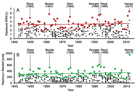
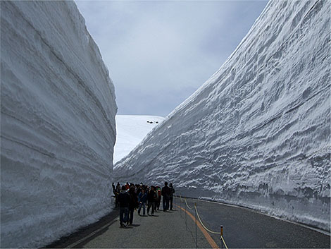
North American meteorologists, welcome to the snow climate of western Japan. Every year in winter lake effect-like snow events bury coastal cities in northern and central Japan under 20-30 feet of snow. Above is the “snow corridor” experienced each spring when the Tateyama Kurobe Alpine Route through the Hida Mountains reopens, revealing the season’s snows in its towering walls. The Hida Mountains, where upwards of 512 inches of snow on average accumulates each winter, are known as the northern Japanese Alps.

The tremendous snow accumulations largely occur from December to February during the East Asian winter monsoon when sea-effect snowbands form behind frequent cold outbreaks. But their snowfall isn’t just pretty to look at and play in — extreme snowfalls combined with dense populations in cities adjacent to the Sea of Japan such as Sapporo (pop. 1.95 million) are public safety hazards, turning exceptionally deadly every year. On average 100 people die and four times that number are injured from snow and ice in Japan, not only from snow removal but also from “roofalanches” — masses of snow sliding off roofs onto people.

Similar to their counterparts downwind of North America’s Great Lakes, the Sea of Japan snowbands invite research from Japanese scientists and those in many other locales where bodies of water enhance snowfall over populated lands. A new paper in BAMS by Jim Steenburgh (University of Utah) et al. not only highlights what’s known about the Japanese snow events but also is designed to “stimulate increased collaborations between sea- and lake-effect researchers and forecasters in North America, Japan, East Asia, and other regions of the world” who can collectively realize the “significant potential to advance our understanding and prediction of sea- and lake-effect precipitation.”

Blending Satellite Imagery is Both ‘Science and Art’ to Maximize Information Delivery

Monitoring the atmosphere by satellite has come a long, long way technologically since TIROS sent back its first snapshots of Earth in 1960. Along with marked advances in spectral, spatial, temporal, and radiometric resolution of state-of-the-art instrumentation, however, come copious volumes of new data as well as unique challenges with how to view it all.

We as users are hardly up to the task alone — there’s insufficient time, especially for operational forecasters. The solution: blended imagery. In short, the seamless display of multivariate atmospheric information gleaned from today’s advanced satellites.

Value-added imagery from NOAA’s GOES-R satellite series, for example, isn’t just useful, but rather at its best it’s “a balance of science and art,” report Steven Miller (Colorado State University) and colleagues of a new paper in the Journal of Atmospheric and Oceanic Technology. Such multidimensional blending of key weather parameters into visually intuitive products maximizes the information available to users.

To illustrate this, the author’s applied the blending technique to new GOES-16’s GEOCOLOR imagery. Below is an example of a “sandwich product” in which (a) color-enhanced infrared imagery with a transparency of 70% is superimposed upon (b) visible reflectance imagery of thunderstorms over Texas, Louisiana, and Arkansas at 2319 UTC April 6, 2018, to dynamically (c) blend the images.

PoN_miller

This “partial transparency” blending technique highlights the overshooting cloud tops in the convection, enabling forecasters to pinpoint the most intense cells. It’s just one of a number of methods the paper highlights to simultaneously display satellite information and thereby present valuable insight.

The technique, Miller et al. state, blurs the line between qualitative imagery users want and quantitative products they need.

To the trained human analyst, capable of drawing context from such value-added imagery, combining the best of both worlds provides a powerful new paradigm for working with the new generation of information-rich satellites.

“Decision-making under meteorological uncertainty” for D-Day’s Famous Forecast

The success of the D-Day Invasion of Normandy was due in part to one of history’s most famous weather forecasts, but new research shows this scientific success resulted more from luck than skill. Oft-neglected historical documentation, including audio files of top-secret phone calls, shows the forecasters were experiencing a situation still researched and practiced today: “decision-making under meteorological uncertainty.”

New research recently published in BAMS into that weather forecast for June 6, 1944, which enabled the Allies in World War II to gain a foothold in Europe, answers questions about three popular perceptions: were the forecasts, which predicted a break in the weather, that good? were the German meteorologists so ill-informed, missing that weather-break? and was the American analog system for prediction so great and better than what the Germans had?

The “alleged” weather break

An expected ridge and fair weather between two areas of low pressure, one departing and one arriving over the area, didn’t materialize. The departing low instead lingered and created a lull in visibility and lifted the cloud ceiling height, but it didn’t slow winds much. They blew at Force 4-5 (~13-24 mph), creating very choppy seas that sickened many troops prior to the invasion.

Synoptic analyses at 00 UTC from 5 to 8 June 1944. The low that was supposed to move northeast to southern Norway remained over the North Sea for some days. On 6 and 8 June the observed winds in the Channel were force 4 and occasionally force 5.
Synoptic analyses at 00 UTC from June 5-8, 1944. The low that was supposed to move northeast to southern Norway remained over the North Sea for some days.


A blown German Forecast?

Because the invasion came as a complete surprise to the Germans it has been surmised their weather forecast for June 6 had to be bad. German forecasters prior to the war were the best at “extended” forecasts, and their synoptic maps and forecast for that day were more realistic than the Allies, with a less optimistic speculation of any break in the weather.

The German's European-Atlantic map at 00 UTC June 6, 1944, where the analysis over the North Atlantic appears not to be based on observations but intercepted American coded analyses.
The German’s European-Atlantic map at 00 UTC June 6, 1944, where the analysis over the North Atlantic appears not to be based on observations but intercepted American coded analyses.


A historically debated forecast

The analog weather prediction system employed by the Allies for the invasion was claimed by its creators to have correctly identified the weather break. But historical analysis and review doesn’t bear this out. What it does find, though, is that the system correctly identified a transition from zonal to meridional flow, which delivered the break the Allies needed for success. History’s finding: The forecast was “Overoptimistic.”

The 1984 Fort Ord meeting about the D-Day forecast got coverage in the local Monterey newspapers. The invasion was said to have occurred in a "break" or a period of a "brief lull" in the weather.
The 1984 Fort Ord, California, AMS meeting about the D-Day forecast got coverage in the local Monterey newspapers. The American forecasting group was led by Lt. Col. (Dr.) Irving Krick of Caltech. The president of the Naval Post Graduate School, Robert Allen, Jr., at the time an Air Force officer conducting high-level weather briefings at the Pentagon, also spoke at the meeting.


As a lesson learned from this most famous of weather forecasts, the paper’s author, Anders Persson of Swedin’s Uppsala University, concludes:

It was 75[+] years ago and the observational coverage has improved tremendously since then, both qualitatively and quantitatively. Our understanding of the atmosphere is much better,and the forecast methods have reached a standard that could hardly have been dreamt of in 1944. However, there’s one element that has a familiar ring to it and is of great interest today. That is when Air Marshall Tedder [Deputy Supreme Commander of the Invasion under General Eisenhower] asks about an assessment of the confidence in the forecast he has just heard … This illustrates that the D-day forecast is a significant early example of decision-making under meteorological uncertainty.

Snowflake Selfies as Meteo Teaching Tools

Undergrads at Penn State recently took to their cellphones to mingle with and snap pics of tiny snowflakes to reinforce meteorological concepts. The class, called “Snowflake Selfies” and described in a new paper in BAMS, was designed to use low-cost, low-tech methods that can be widely adapted at other institutions to engage students in hands-on field research.

In addition to photographing snow crystals, students measured snowfall amounts and snow-to-liquid ratios, and then gained meteorological insight into the observations using radar data and thermodynamic soundings. The goal of the course was to reinforce concepts from their other undergraduate meteorology courses, such as atmospheric thermodynamics, cloud physics, and radar and mesoscale meteorology.

As a writing intensive course at Penn State that meets the communication skills requirement of the AMS guidance for a Bachelor’s Degree in Atmospheric Science, “Snowflake Selfies” also was designed to help students communicate meteorological science. Students shared their observations with the local National Weather Service office in State College and also wrote up their work in term papers and presented their pics and findings to the class.

Snow crystal photographs taken by students in the "Snowflake Selfies" class.
Snow crystal photos taken by students in the “Snowflake Selfies” class.


Of course to have such a class, you need snow, and “the relative lack of snowfall events during the observational period” in winter 2018 was definitively a challenge for students, the BAMS paper states. Pennsylvania’s long winters often see many opportunities to photograph snow, but the course creators caution that perhaps a longer observational period is needed in case nature doesn’t cooperate. It also would allow students enough time to closely observe snowflakes while juggling their other classes and activities.

A survey conducted at the end of the class found that “Snowflake Selfies” was well received by students, engaging them and encouraging their introduction to field science. And they “strongly agreed [it] helped reinforce their understanding of cloud physics and physical meteorology compared to” a previous such course where students designed, built, and deployed their own 3-D printed rain gauges to measure precipitation.

Actually, that previous course sounds like a lot of fun, too!

Observations without Fear: NOAA’s Drones for Hurricane Hunting

Nowhere is it more dangerous to fly in a hurricane than right near the roiling surface of the ocean. These days, hurricane hunting aircraft wisely steer clear of this boundary layer, but as a result observations at the bottom of the atmosphere where we experience storms are scarce. Enter the one kind of plane that’s fearless about filling this observation gap: the drone.

NOAA’s hurricane hunter aircraft in recent storms has been experimenting with launching small unmanned aircraft systems (sUAS) into raging storms–and these devices show promise for informing advisories as well as improving numerical modeling.

Lead author Joe Cione of NOAA's hurricane research division holds a Coyote sUAS. The drones are being launched into hurricanes from the P-3 hurricane hunter aircraft in the background.
Lead author of a new paper in BAMS, Joe Cione of NOAA’s Hurricane Research Division, holds a Coyote sUAS. The drones are being launched into hurricanes from the WP-3D Orion hurricane hunter aircraft in the background.


The observations were made by a new type of sUAS, described in a recently published paper in BAMS, called the Coyote that flew below 1 km in hurricanes. Sampling winds, temperature, and humidity in this so-called planetary boundary layer (PBL), the expendable Coyotes flew as low as 136 m in wind speeds as high as 87 m s-1 (196 mph) and for as long as 40 minutes before crashing (as intended) into the ocean.

In the BAMS article, Joe Cione at al. describe the value of and uses for the low-level hurricane observations:

Such high-resolution measurements of winds and thermodynamic properties in strong hurricanes are rare below 2-km altitude and can provide insight into processes that influence hurricane intensity and intensity change. For example, these observations—collected in real time—can be used to quantify air-sea fluxes of latent and sensible heat, and momentum, which have uncertain values but are a key to hurricane maximum intensity and intensification rate.

Highs-lows

Coyote was first deployed successfully in Hurricane Edouard (2014) from NOAA’s WP-3 Orion hurricane hunter aircraft. Recent Coyote sUAS deployments in Hurricanes Maria (2017) and Michael (2018) include the first direct measurements of turbulence properties at low levels (below 150 m) in a hurricane eyewall. In some instances the data, relayed in near real-time, were noted in National Hurricane Center advisories.

Turbulence processes in the PBL are also important for hurricane structure and intensification. Data collected by the Coyote can be used to evaluate hurricane forecasting tools, such as NOAA’s Hurricane Weather Research and Forecasting (HWRF) system. sUAS platforms offer a unique opportunity to collect additional measurements within hurricanes that are needed to improve physical PBL parameterization.

Coyote launch sequence: (a) Release in a sonobuoy canister from a NOAA P-3. (b) A parachute slows descent. (c) The canister falls away and the Coyote wings and stabilizers deploy. The main wings and vertical stabilizers have no control surfaces; rather, elevons (i.e., combined elevator and aileron) are on the rear wings, controlled by the GPS-guided Piccolo autopilot system with internal accelerometers and gyros. (d) After the Coyote is in an operational configuration, the parachute releases. (e) The Coyote levels out after starting the electric pusher motor, which leaves minimally disturbed air for sampling at the nose. The cruising airspeed is 28 m s-1. (f) The Coyote attains level flight and begins operations. When deployed, the Coyote’s wingspan is 1.5 m and its length is 0.9 m. The 6-kg sUAS can carry up to 1.8 kg. Images were captured from a video courtesy of Raytheon Corporation.
Coyote launch sequence: (a) Release in a sonobuoy canister from a NOAA P-3. (b) A parachute slows descent. (c) The canister falls away and the Coyote wings and stabilizers deploy. The main wings and vertical stabilizers have no control surfaces; rather, elevons (i.e., combined elevator and aileron) are on the rear wings, controlled by the GPS-guided Piccolo autopilot system with internal accelerometers and gyros. (d) After the Coyote is in an operational configuration, the parachute releases. (e) The Coyote levels out after starting the electric pusher motor, which leaves minimally disturbed air for sampling at the nose. The cruising airspeed is 28 m s-1. (f) The Coyote attains level flight and begins operations. When deployed, the Coyote’s wingspan is 1.5 m and its length is 0.9 m. The 6-kg sUAS can carry up to 1.8 kg.
Images were captured from a video courtesy of Raytheon Corporation.


The authors write that during some flights instrument challenges occurred. For example:

thermodynamic data were unusable for roughly half of the missions. Because the aircraft are not recovered following each flight, the causes of these issues are unknown. New, improved instrument packages will include a multi-hole turbulence probe, improved thermodynamic and infrared sensors, and a laser or radar altimeter system to provide information on ocean waves and to more accurately measure the aircraft altitude.

Future uses of the sUAS could include targeting hurricane regions for observations where direct measurements are rare and models produce large uncertainty. Meanwhile, the article concludes, efforts are underway to increase sUAS payload capacity, battery life, and transmission range so that the NOAA P-3 need not loiter nearby.