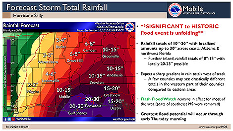
Hurricane Sally is inching ashore in southeast Alabama Wednesday morning and has started to flood parts of the central Gulf Coast with an expected 1-2 feet of rain, maybe more. With that much rain forecast, it seems likely to join other recent catastrophic flood disasters Harvey (2017) and Florence (2018) in ushering in a new era of rainier storms at landfall that bring with them an extreme rain and flooding threat.
And with more wetter storms on the way, better communication about these potentially deadly impacts from copious rainfall is needed. Another BAMS article we blogged about addressed this by creating an Intuitive Metric for Deadly Tropical Cyclone Rains. Its authors designed the new tool—the extreme rainfall multiplier (ERM)—to easily understand the magnitude of life-threatening extreme rain events.
Co-author James Kossin explained to BAMS:
Water presents a much greater hazard in a hurricane than wind does, but the Saffir-Simpson categories are based on wind-speed alone. Salt-water hazards along and near the coast are caused by storm surge. Coastal residents are warned about these hazards and are provided with evacuation plans. Fresh-water flooding from extreme hurricane rainfall, however, can happen inland away from evacuation zones, and pose the greatest threat to life and property in these areas where people tend to shelter-in-place. Compound hazards such as dam failures and land-slides in mountainous regions pose additional significant threats. In this case, effective warnings and communication of the threats to inland populations is paramount to reduce mortality. This work strives to present a tool for providing warnings based on people’s past experience, which gives them a familiar reference point from which to assess their risk and make informed decisions.
Lead author Christopher Bosma:
We started out this project focused on analyzing the catastrophic and record-breaking rainfall associated with Hurricane Harvey. But, as we started to finish our analysis of that system, just a year later, Hurricane Florence brought devastating and torrential rainfall to the Carolinas, which forced us to go back and revisit some of our initial analysis. The fact that multiple major storms happened in quick succession grabbed a lot of headlines, but, from a research and scientific perspective, it also provided a chance to note how the messaging used to describe these systems had changed (or not) and think of other ways to use the metric we had developed.
ERM is not yet operational, but that is the researchers’ goal, to “convey effective warnings to people about fresh-water flooding threats,” Kossin says.
Hurricane Sally is one such extreme rainfall flood threat, with “significant to historic flooding” likely, the National Weather Service says.
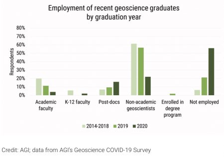
A new survey by the American Geosciences Institute shows that recent graduates in the geosciences are finding employment at the same rates as before the COVID-19 pandemic, but a separate survey from Nature finds that amid tightening funding science postdocs are nervous about ongoing research as well as career opportunities.
The AGI survey covered graduates from the classes of 2018, 2019, and 2020, and found no “deviation from long-term employment trends of recent geoscience graduates.”
As of August 2020, 94% of geoscience graduates who earned their degree between 2014-2018 were employed, while 77% of graduates from 2019 and 44% of graduates from 2020 reported the same. For geoscience graduates who earned their degree this year, 16% of bachelor’s, 57% of master’s, and 91% of doctorates have secured employment.
For comparison, data from the 2013-2018 AGI Geoscience Exit Survey shows that 20% of geoscience graduates secured employment by the time they graduated. This data varied by degree level, with 12% of bachelor’s, 36% of master’s, and 56% of doctorates securing employment by the time they graduated. Only 1% of employed recent geoscience graduates lost their job since February 2020.
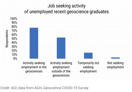
While three-quarters of the still-unemployed graduates of the last three classes were still looking for jobs in the geosciences, half said they were instead, or additionally, now seeking employment outside the field. Of those seeking employment outside the field, more than 80% said this was due to lack of jobs in the geosciences, and about three-quarters felt they did not have sufficient training for the available jobs.
The AGI employment statistics are provided by geoscience graduate job seekers, part of a series AGI is publishing on the effects of the pandemic in the geosciences. The Nature survey, by contrast, sampled views of postdocs worldwide and “paints a gloomy picture of job-loss fears, interrupted research, and anxiety about the future.” It finds that:
Eight out of ten postdoctoral researchers say that the global coronavirus pandemic has hampered their ability to conduct experiments or collect data. More than half are finding it harder to discuss their research ideas or share their work with their laboratory head or colleagues, and nearly two-thirds believe that the pandemic has negatively affected their career prospects.
The pandemic has shuttered or reduced the output of academic labs globally, slashed institutional budgets and threatened the availability of grants, fellowships and other postdoctoral funding sources. The fallout adds up to a major challenge for a group of junior researchers who were already grappling with limited funds, intense job competition and career uncertainties.
The Nature survey drew responses from 7,670 postdocs working in academia from mid-June through the end of July. Some respondents were selected for follow-up interviews, which “filled in an unsettled, precarious picture of postdoctoral research in the era of coronavirus.”
“The [pandemic] has compounded the pressures that postdocs were already under,” reported one of the interviewees, Hannah Wardill, a cancer researcher at the South Australian Health and Medical Research Institute in Adelaide.
Derechos are less common than Midwestern tornadoes, but occur almost every year in that region as well as other parts of the United States. Yet they remain exotic and mystifying. Even to meteorologists.
The reason appears to lie in the complex way the long-lived windstorms form. Derechos are often incorrectly referred to as inland hurricanes; their damaging winds can reach hurricane force, but they are straight-line in nature, rather than circulating around a common center. When people suffer, though, they can be forgiven for using the wrong windstorm term. By definition derechos have to meet specific criteria, such as causing damage continuously or intermittently in a lengthy line of at least 400 miles that’s at least 60 miles wide. But just like hurricanes, they come in a variety of intensities.
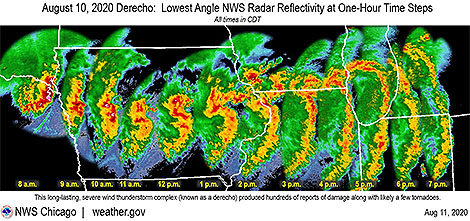
Last week’s derecho, roaring 750 miles from eastern Nebraska across Iowa, Illinois and Indiana, was particularly ferocious with winds in multiple swaths across Iowa gusting to over 100 mph. The National Weather Service found damage to an apartment complex in Cedar Rapids, Iowa, consistent with wind gusts of an astonishing 130-140 mph. But even these extreme winds and the severe damage they wrought don’t tell the whole story of the variation in these windy storms with the seemingly odd name.
The AMS Glossary of Meteorology states: “The term derecho derives from a Spanish word that can be interpreted as “straight ahead” or “direct” and was chosen to discriminate between wind damage caused by tornadoes, which have rotating flow, from straight-line winds.” It defines derechos as widespread convectively induced straight-line windstorms.
Two Very Different Derechos: Base reflectivity composite radar data for (a) 2056 UTC 4 Apr 2011 and (b) 2234 UTC 29 Jun 2012, with surface observations plotted using conventional station plot format. Convective system in (a) is composed of a series of loosely connected, largely linear bands with low-amplitude LEWPs, whereas that in (b) consists of a single, intense arc of storms with a well-defined bow echo. Animated radar and satellite imagery for these events may be viewed at http://spc.noaa.gov/misc/AbtDerechos/casepages/apr042011page.htm and http://spc.noaa.gov/misc/AbtDerechos/casepages/jun292012page.htm.
This updated definition was the work of a team of meteorologists about five years ago who compared different straight-line windstorms—all meeting the damage criteria of derechos at the time but clearly having different mechanisms driving them. Their published paper in the Bulletin of the American Meteorological Society was “A Proposed Revision to the Definition of ‘Derecho’.” With it, the authors made the case to improve the definition of derecho to make it more physically based and more closely mirror other definable meteorological terms such as tornadoes, extratropical cyclones, and cirrus clouds.
While the paper had a positive effect among the meteorological community, a web search still turns up different definitions of derecho among meteorological websites, including within the NWS.
We asked the lead author of the BAMS paper, Stephen Corfidi (NOAA NWS, CIMMS, University of Oklahoma), for his thoughts on last week’s Midwestern derecho, to put it in perspective and also to help explain the reasons behind the difficulty with meteorologists not only defining but using the meteorological term differently.
BAMS: Was last week’s Midwest fast-moving line of severe thunderstorms with damaging winds a derecho? If so, did it fit the Glossary definition of a derecho?
Stephen Corfidi: Last Tuesday’s Midwest wind storm met the AMS Glossary definition of a derecho. Most significantly, it satisfied the criterion for the presence of “one or more sustained bow echoes with mesoscale vortices and/or rear-inflow jets.” A large mesoscale vortex, located on the north end of the larger-scale bow-shaped convective system from central Iowa to Lake Michigan, appears to have been associated with some of the strongest and longest-duration surface winds that accompanied the event. While the swath of organized damaging winds was not particularly long (on the order of 500 miles (800 km)) in comparison to some past events, the length well exceeded the somewhat flexible 400-mile (~ 650 km) cut-off used to distinguish derecho storms.
BAMS: Among derechos, how does this one rank?
SC: The Iowa-Illinois storm is certainly one of the most memorable of 2020—a year that already has seen other noteworthy events (e.g., those in Colorado, the Dakotas, and Pennsylvania in June). What made the Iowa-Illinois event especially noteworthy was the sizable number of reliably-observed significant surface gusts. There were numerous reports in excess of 80 mph (35 meters/second), and incidental evidence that some locations experienced speeds greater than 100 mph (45 m/s). The strong winds—likely enhanced by the presence of the mesoscale vortex—in some places persisted for more than 30 minutes. The vortex to some extent resembled the “warm-core” (hurricane-like) circulation that formed within the Kansas-Missouri-Illinois derecho of 8 May 2009.
BAMS: What made this one stand out?
SC: The duration of the storm’s high winds over eastern Iowa and western Illinois—again, likely due in part to the presence of the large mesoscale vortex—was certainly outstanding. This is quite a statement considering that the event occurred in a region known for its propensity for derechos (Recall that Gustave Hinrich’s nineteenth century studies of straight-line wind events were based in Iowa).
BAMS: Why are derechos so perplexing and difficult for meteorologists to acceptably define?
SC: There are several reasons why derechos are not only difficult to define, but also challenging to forecast. Unlike supercell thunderstorms that, in most cases, are well-delimited in time and space, broad swaths of damaging convective winds can arise in many different ways. Some of the processes involved in derecho development remain poorly understood and / or are only partly resolved by current observational platforms.
More significantly, unlike weather phenomena like supercells, derechos may or may not be accompanied by meteorological structures that readily are apparent to human observers. For example, most meteorologists recognize a supercell when one appears in the sky. But specific cloud formations are not associated with derechos, and the characteristic meteorological structures that do accompany many derechos (e.g., embedded vortices and rear-inflow jets) are too large or subtle to be recognized by human observers without the aid of remote-sensing devices such as radar and satellite.
These same aspects make derechos difficult to forecast. One can say that derechos arise when a unique combination of known and unknown necessary ingredients is present over a sufficiently broad area to support rapid, repetitive, downshear thunderstorm development. That said, applying this concept in practice presents a formidable challenge. In some cases, the known ingredients are present, but the extent of the favorable environment is too limited for derecho status to be realized. Conversely, expansive environments sometimes appear that are supportive of widespread destructive winds, but not those strongly dependent on the smaller-scale processes associated with rear-inflow jets and mesoscale vortices.
As with any weather forecast, when “missed” derecho events occur, the root causes can be traced to the existence of too many unknowns—both observational and theoretical. In the case of derechos, both unknowns, at present, remain sizable.
BAMS: What has been the impact of your 2016 BAMS paper and proposed new definition?
SC: It does appear that the updated definition proposed in the paper has been adopted to at least some extent in the severe weather community; the updated definition in the AMS’ Glossary likely abetted the effort. There is, of course, no “official” arbiter of general meteorological terms. This explains, in part, the range of derecho “definitions” that appear in some sources. The lack of consistency in the use of the term “derecho” was, in fact, a motivating factor in drafting the paper. We’d like to think that the paper focused needed attention on the value of increased precision in meteorological terminology, but that is not something that is easy to measure. It is probably safe to say that the definition of “derecho” will continue to change as the underlying processes responsible for the most intense storms become better understood.
BAMS: What would you like readers of your 2016 paper to learn about and from the re-defining of derecho?
SC: I think perhaps the most important take-aways are that (1) the existing definition was outdated because of the significant changes that have occurred in observational data, record-keeping, and understanding since the mid-1980s, and (2) that if we are to better understand and forecast high-wind-producing convective systems, we need to first better classify those systems that are observed.
BAMS: You and your colleagues at NOAA-NWS-NCEP put together a comprehensive and impressive website About Derechos. How did you become interested in them?
SC: Convective systems, in general, are interesting because there are so many “moving parts” involved in their development, sustenance, and motion. It is especially challenging—but also rewarding—to try to assess the strength and likely longevity of those processes in real-time so as to prepare useful forecasts. Derechos are high-impact events; they are one area where society would benefit greatly from increased meteorological knowledge.
BAMS: What was the biggest challenge you encountered in your work to update the derecho definition?
SC: Having thoughts on introducing any new idea is one thing, but putting those concepts into words is another. Unlike most other papers in our “business,” in this one I felt we had to be somewhat persuasive. I was not at first comfortable with taking such an approach. But the contrasts presented by the two derecho events introduced in the first part of the paper furthered my conviction that persuasion was needed to both defend and encourage discussion on the definition topic.
BAMS: What got you initially interested in meteorology?
SC: My interest in clouds and storms goes back to my earliest days as a young kid growing up in a house kept super-clean by my mom. Because I was forbidden to play in the yard when the grass was wet (I’d track dirt into the house, of course!), I soon came to appreciate “Mr. Sun.” In particular, I noticed that I’d often not see the sun the next day if certain cloud formations had appeared in the sky on the previous one. A bit later, in first grade, my dad introduced me to weather books in the local library. Some had cloud pictures indicating which formations were “bad,” and which were associated with good weather. I was hooked! Thunderstorm days were always a favorite because the clouds on such days seemed to change the most rapidly—and provided the most surprises. I was very interested in things like rocks and plants, too—but weather was always #1.
Through July, 2020 has been on almost the same track as 2016: the two years had the hottest first seven months in NOAA’s 141 year dataset of global surface temperatures (land and ocean combined). Since 2016 turned out to be the hottest year on record, it might seem as if this fast start puts 2020 on track to set a new record, too, or to be a near miss. NOAA says it’s already “very likely” 2020 will be among the five hottest years on record.
But in the strange reality of ever rising global temperatures, it’s not so much the first half of the year that puts 2020 on the verge of a record. It’s the underlying trend of warming: 2020 was already on the verge on New Year’s Day.
As the new State of the Climate in 2019 released last week points out, the six hottest years in the last century and a half were…exactly the last six years, 2014-2019. Due to global warming, practically every year’s surface temperature is going to be a hot one. Just by showing up at the starting line, every year is a serious threat to set a new standard.
The study, by Anthony Arguez (NOAA/NCEI) et al. also finds an 82% chance that all years in the next decade will rank in the top 15 warmest years as global warming continues. Its authors suggest that record warm years are already “baked into the cake” of Earth’s global climate and that it would take “an abrupt climate shift for even a few years within the next decade to register outside the top 10 warmest years.”
To determine these odds, the researchers analyzed the monthly version of NOAA’s Merged Land Ocean Global Surface Temperature Analysis Dataset (NOAAGlobalTemp) to project annual global temperature rankings in the future. The ever-shifting expectations for global temperatures render the usual way of keeping tabs on the data—by comparing to 30-year normals—inadequate. So Arguez et al. formulated a new way to compare each year to surrounding years:
We introduce a “temperature score” to help NOAA communicate the coolness or warmth of a given year relative to the long-term trend. We believe this is the first such projected ranking and temperature score currently produced operationally. Our objective is to use this tool to improve the communication of climate change impacts to the general public.
The temperature score from 1 (a very cold year) to 10 (very warm) is useful to distinguish between warmer and colder years relative to the long-term trend. As examples, the authors note that 2008 and 2011 were considerably cooler than surrounding years and below the overall trend, whereas 1998 and 2016 were not only the warmest years on record but were also notably warmer than surrounding years.
The study only includes average annual global temperatures through 2018. But as reported in the annual State of the Climate, 2019 ranks as the second or third warmest year on record (depending on your favored dataset), adding another year to the recent string of those warmer than any years back to the mid 1800s. The report notes that each successive decade since 1980 has been warmer than the previous. Arguez’ research suggests that not only will this continue but it will worsen dramatically.
This is a testament to the exceptional warmth experienced over the last few decades, punctuated by the last [5] years [2015–19], which have separated themselves from “the pack.”
We asked Arguez a few questions (more found in the latest print/digital issue of BAMS) about this work as well as about his background and what sparked his interest in meteorology.
BAMS: What would you like readers to learn from your study of record global temperatures?
Anthony Arguez: I would like the general public to know that there is not a great deal of suspense that most years—if not all—over the next decade will likely register as top 10 years. In fact, the data suggest we should expect this, as it would likely take a pretty abrupt change to get us off this trajectory.
BAMS: How did you become interested in finding new ways to analyze the global temperatures and their trend?
AA: I feel like I’ve been staring at the annual global temperature time series continually over the past 15 years or so because it is just so interesting in many ways. I find it challenging and rewarding to develop methods to translate volumes of data into answers to specific questions posed by the general public. I’ve drawn inspiration from Nate Silver, whose penchant for expounding on and communicating the “signal” hidden in the “noise” informs the way I would like to see myself and fellow climate scientists communicate to the general public more effectively.
BAMS: What surprised you most in doing this work?
AA: I was very surprised that the ranking errors we found were so small! Before calculating the results, I had a gut feeling that these errors would be modest, but the mean absolute ranking error of ~2 spots a full 10 years out was well below anything I could have imagined. I clearly under-appreciated the predictability inherent in the observed upward trend when it comes to annual global temperature rankings.
BAMS: What was the biggest challenge?
AA: I think the biggest challenge we faced was that we were not aware of any similar operational products in existence (neither for projected rankings or global annual temperature scores), or of any papers that had characterized ranking errors in a similar fashion, so we were in uncharted territory to some extent.
BAMS: This isn’t the biggest climate challenge, or surprise, you’ve ever faced…
AA: I became interested in meteorology as a teenager in 1992 when Hurricane Andrew totaled my parents’ home in Miami, Florida.
Today’s publication of State of the Climate in 2019 marks the 30th annual release in this series of supplements to the Bulletin of the American Meteorological Society. The report is not just a service for immediate use as the latest status report on climate. It’s a resource that people worldwide will use throughout the year, and indeed as a reference through the coming years. The report, now online only, is meant to stand a test of time as a bedrock of other reports and decisions. Despite the rapid pace of writing, editing, and reviewing, this is obviously not the first (or last) assessment of 2019’s climate. So we still often get asked—why now? Why release in August 2020 a comprehensive, validated check-up on the health of our planet’s climate in 2019 August, instead of in January, when it’s still hot news?
Co-editor Jessica Blunden of NOAA addressed the question a number of years ago, with a helpful look behind the scenes of State of the Climate. You can appreciate, first of all, the amazing job she and coeditor Deke Arndt (also of NOAA) do to pull this all together so fast—they’re coordinating the work of more than 500 authors and chapter editors from 61 different countries. So naturally, at first glance, churning out this report in only a matter of months is a managerial triumph–a testament to international cooperation:
The production of this document really does “take a village”; without the dedication and hard work of every single one of the people who contribute to this process, the quality and scope of the report would not be possible. Each year the number of authors tends to increase as we add new information to the report.
In just the past decade alone Blunden and Arndt have added 150 authors and 13 additional countries. Why so many authors?
The authors are asked to contribute based on their expertise in a specific field. For our Regional Climates chapter, which is comprised of annual summaries for countries around the world, the authors are often affiliated with a specific country’s official meteorological/hydrological agency and provide analysis based on data from that agency. it’s not just any process of coordination. State of the Climate is an elaborate scheme to make a scientifically worthwhile document:
The development of the report is quite rigorous, with writing, two major peer-review processes, technical editing, layout, and approval. After the calendar year has ended, authors are given about six weeks to develop their content and provide an initial draft that is reviewed by the chapter editors.
Then the chapter editor has the draft reviewed by two or three scientists with expert knowledge in that field. Generally, we allow one to two weeks for this review to be completed and another one to two weeks for the authors to make revisions, as needed, and for the chapter editors to prepare the new version for a formal, external review.
The external review process involves anonymous peer reviews, and BAMS allows three weeks for these reviews to be completed. The authors and chapter editors then have two weeks to make revisions based on these comments and submit the final draft for approval.
Then there’s editing and layout and so on . . . as Blunden summarizes:
This document takes the time to provide the most accurate information available on the state of the climate system.
But the time isn’t actually about writing and reviewing; it’s the comprehensiveness of 429 pages and a bazillion references (no, we didn’t count them). A report that started as a 30-pager gets bigger and more precise with each iteration, because the value increases:
The longer a data record is and the larger the area it covers, the more useful it is for putting a particular climate indicator into context, for example comparing one year to another, or detecting trends over time. Today we are fortunate to have technologies and capabilities that were not available to us decades ago, such as satellite observations, but to use all those observations for climate research means combining observations from multiple sources into a single, seamless climate data record, which is neither fast nor easy.
With both satellite and direct observations, it is important to reconcile data discrepancies and inaccuracies so that the climate records are correct, complete, and comparable, and this painstaking process can take years. For our report, a high-quality dataset is ready for inclusion only after its development processes and methodologies have been scrutinized through peer review with published results. That way readers of the State of the Climate reports can depend on detailed journal articles if they want to understand the details of a data record.
The process of creating a climate quality data set and then having it evaluated by other scientists through peer review is so challenging, no more than a few are added to the State of the Climate report each year.
So the State of Climate is a testament to a complex process, with complex, interrelated data sources that cry out for the reconciliation and comparison that makes the report unique. And of course, all about a climate that is nothing if not the paragon of complexity.
As Deke Arndt explains about Earth’s climate (in a webinar to watch before using State of the Climate): “If the Earth didn’t spin, and we didn’t have day and night, it would be very simple.”
That sums up the reason the State of the Climate is not simple . . . or small, or fast. It is all connected.
Today’s publication of State of the Climate in 2019 marks the 30th annual release in this series of supplements to the Bulletin of the American Meteorological Society. The report is not just a service for immediate use as the latest status report on climate. It’s a resource that people worldwide will use throughout the year, and indeed as a reference through the coming years. The report, now online only, is meant to stand a test of time as a bedrock of other reports and decisions.
Despite the rapid pace of writing, editing, and reviewing, this is obviously not the first (or last) assessment of 2019’s climate. So we still often get asked—why now? Why release in August 2020 a comprehensive, validated check-up on the health of our planet’s climate in 2019 August, instead of in January, when it’s still hot news?
Co-editor Jessica Blunden of NOAA addressed the question a number of years ago, with a helpful look behind the scenes of State of the Climate. You can appreciate, first of all, the amazing job she and coeditor Deke Arndt (also of NOAA) do to pull this all together so fast—they’re coordinating the work of more than 500 authors and chapter editors from 61 different countries. So naturally, at first glance, churning out this report in only a matter of months is a managerial triumph–a testament to international cooperation:
The production of this document really does “take a village”; without the dedication and hard work of every single one of the people who contribute to this process, the quality and scope of the report would not be possible. Each year the number of authors tends to increase as we add new information to the report.
In just the past decade alone Blunden and Arndt have added 150 authors and 13 additional countries. Why so many authors?
The authors are asked to contribute based on their expertise in a specific field. For our Regional Climates chapter, which is comprised of annual summaries for countries around the world, the authors are often affiliated with a specific country’s official meteorological/hydrological agency and provide analysis based on data from that agency. it’s not just any process of coordination. State of the Climate is an elaborate scheme to make a scientifically worthwhile document:
The development of the report is quite rigorous, with writing, two major peer-review processes, technical editing, layout, and approval. After the calendar year has ended, authors are given about six weeks to develop their content and provide an initial draft that is reviewed by the chapter editors.
Then the chapter editor has the draft reviewed by two or three scientists with expert knowledge in that field. Generally, we allow one to two weeks for this review to be completed and another one to two weeks for the authors to make revisions, as needed, and for the chapter editors to prepare the new version for a formal, external review.
The external review process involves anonymous peer reviews, and BAMS allows three weeks for these reviews to be completed. The authors and chapter editors then have two weeks to make revisions based on these comments and submit the final draft for approval.
Then there’s editing and layout and so on . . . as Blunden summarizes:
This document takes the time to provide the most accurate information available on the state of the climate system.
But the time isn’t actually about writing and reviewing; it’s the comprehensiveness of 429 pages and a bazillion references (no, we didn’t count them). A report that started as a 30-pager gets bigger and more precise with each iteration, because the value increases:
The longer a data record is and the larger the area it covers, the more useful it is for putting a particular climate indicator into context, for example comparing one year to another, or detecting trends over time. Today we are fortunate to have technologies and capabilities that were not available to us decades ago, such as satellite observations, but to use all those observations for climate research means combining observations from multiple sources into a single, seamless climate data record, which is neither fast nor easy.
With both satellite and direct observations, it is important to reconcile data discrepancies and inaccuracies so that the climate records are correct, complete, and comparable, and this painstaking process can take years. For our report, a high-quality dataset is ready for inclusion only after its development processes and methodologies have been scrutinized through peer review with published results. That way readers of the State of the Climate reports can depend on detailed journal articles if they want to understand the details of a data record.
The process of creating a climate quality data set and then having it evaluated by other scientists through peer review is so challenging, no more than a few are added to the State of the Climate report each year.
So the State of Climate is a testament to a complex process, with complex, interrelated data sources that cry out for the reconciliation and comparison that makes the report unique. And of course, all about a climate that is nothing if not the paragon of complexity.
As Deke Arndt explains about Earth’s climate (in a webinar to watch before using State of the Climate): “If the Earth didn’t spin, and we didn’t have day and night, it would be very simple.”
That sums up the reason the State of the Climate is not simple . . . or small, or fast. It is all connected.
Even tall tales have their facts, but in historical fiction the myriad factual details often far outshine the story itself. In the ever popular books of Laura Ingalls Wilder, the telling details turn out to be the truly epic—and real—weather of the past. Barbara Mayes Boustead (University of Nebraska—Lincoln) and her coauthors show us in a recent BAMS article that Wilder’s, The Long Winter, isn’t just good history wrapped into a great novel–it’s also valuable climate data.
The cold, snowy season of 1880-81 featured in The Long Winter was strikingly difficult across much of the Plains and Midwest. A number of accounts have referred to it as the “Hard Winter” or “Starvation Winter.” Wilder’s story, set in De Smet, Dakota Territory (present-day South Dakota; 60 km west of Brookings), is fiction, but it contains many verifiable facts about the weather.
Boustead and co-authors Martha D. Shulski and Steven D. Hilberg set out to determine which parts of Laura’s stories are based in fact, and in the process, filled in the gap left by the absence of analysis or documentation in scientific literature about the Hard Winter of 1880-81. In the process, Boustead et al. show that the Hard Winter places recent severe winters, such as 2013-14, into context.
The winter began early, with a blizzard in eastern South Dakota and surrounding areas in mid October. Following a respite thereafter, wintry conditions returned by mid-November, followed by a number of snow and potential blizzard events in December. After a cold but relatively snow-free period, storm frequency increased from early January through February, producing snow almost daily in eastern South Dakota. In March, most days remained below freezing, though snowfall frequency decreased. Cold conditions continued into the first half of April. The BAMS article goes into detail describing why the winter of 1880-81 was so severe.
BAMS asked a few questions of Boustead to gain insight into her research. A sampling of answers are below:
BAMS: What would you like readers to learn from your article?
Barbara Mayes Boustead: Literature and other creative work can provide windows into past weather events and climates – including everything from documentary evidence to the impacts of those events on individuals and communities. We can connect those works to other historical weather data sources, from observations to reanalysis data, to reconstruct what occurred during these noted events, and why. By researching weather and climate related to a popular-interest subject like Laura Ingalls Wilder and the Little House stories, I have been able to reach audiences that otherwise might not have been so engaged, sparking interest in weather and climate by presenting it through Laura’s perspective.
BAMS: How did you become interested in investigating the weather of Wilder’s book?
Barbara Mayes Boustead: The Long Winter research began over a decade ago as I reread the book as a “comfort read” on the tail end of a winter, reminding myself that even the longest winters do eventually end. I’ve been reading Laura Ingalls Wilder’s books since I was in elementary school, and I had always wondered if the winter was really as Wilder had described it. And then I got to thinking – I am a meteorologist, and I have the tools to look it up! The deeper I dug, the more that my questions led to more questions. I especially got excited as I found data that verified much of the weather that Wilder had described. And I knew I had found a resonant topic when I presented the work at a conference called LauraPalooza in 2010 (it’s real and it’s serious!) and was overwhelmed with questions and discussion following my presentation.
BAMS: What got you initially interested in weather and, more importantly, these novels?
Barbara Mayes Boustead: It seems that many meteorologists started with either a memorable event or a fear of a weather phenomenon. I was in the latter group, afraid of thunderstorms in my preschool years. My mother and sister took me to the library so that I could read books about weather, hoping that understanding would help me conquer fear. I had plowed through all of the books in the library in about a year, and I was hooked! As for my interest in Laura Ingalls Wilder, I can again thank my mom and books. She purchased Little House on the Prairie for me at a garage sale when I was in first grade and ready for chapter books. I turned my nose up at it, but she encouraged me to give it a chance. I did, and of course, Mom knows best – I was hooked and plowed through the rest of the book series, too.
BAMS: What surprised you the most in doing this research?
Barbara Mayes Boustead: Laura Ingalls Wilder was an excellent weather observer. Having researched the winter of 1880-81 extensively, as well as the rest of the identifiable weather and climate phenomena throughout the Little House books, I found that while many elements of the books were fictionalized, she recounted weather and climate events with great accuracy. Almost every weather or climate detail in her books really did occur and usually occurred just as she described it. She occasionally moved some timelines around, but the events themselves were spot-on.
BAMS: What was the biggest challenge you encountered in the research?
Barbara Mayes Boustead: There were times during my research that I would have gone to great lengths to obtain true snowfall measurements from one of the observing sites near the area of interest, or to fill in the spatial gaps. Snowfall data just don’t exist for the central U.S. in the early 1880s.
BAMS: What’s next?
Barbara Mayes Boustead: Research into the weather and climate of Laura Ingalls Wilder’s books and life continues as I work to document other weather and climate events from her other books and stories. Given the popular interest in Laura Ingalls Wilder, some of the research is and will be written for broader audiences, providing a window into the world of science (meteorology and climatology) for non-specialists by standing on the shoulders of Laura Ingalls Wilder’s storytelling and characters. What began as a side project has transitioned into decades worth of research and storytelling! Her books include everything from tornadoes and hail storms to blizzards, droughts to floods, extreme cold to extreme heat. There is fodder for research for years to come!
Thursday NOAA updated its forecast to an “extremely active” Atlantic hurricane season. That has some news outlets linking the 19-25 predicted named storms to Earth’s future—even warmer—global climate. The future looks like it will indeed bring high levels of overall “activity” due to the intense, damaging hurricanes of a warming world (regardless of whether the frequency of storms overall changes). And, of course, settling into a new “norm” isn’t going to happen while warming is ongoing. But the huge number of storms forming? That’s a lot of what the public takes away from the forecast, and that profusion of named storms is not projected to be characteristic of seasons to come.
As we blogged here in May, recent research published in the Bulletin of the American Meteorological Societyfinds there’s no evidence to support an increasing trend in tropical cyclone frequency. In that assessment of the current literature, Tom Knutson (NOAA) and other top tropical experts reviewed a number of peer-reviewed studies and determined that a majority found the numbers of named storms actually decrease in climate projections as we move deeper into this century. But there was no consensus among the authors to either support or refute those studies since their research also showed that “there is no clear observational evidence for a detectable human influence on historical global TC frequency.”
Their assessment did find that we can expect stronger and wetter hurricanes in our warming world and, notably, a possible uptick in the number of intense (Category 4 and 5) hurricanes. It’s these storms that have Knutson and his colleagues most concerned since a majority of hurricane damage is done by the big ones. Their increase is alarming even if the number of storms goes down.
Notable with this week’s forecast update is a prediction close to record territory. “We’ve never forecast up to 25 named storms” before—more than twice a season’s typical 12—noted Jerry Bell, lead seasonal hurricane forecaster at NOAA’s Climate Prediction Center. He went on to say there will be “more, stronger, and longer-lived storms than average” in the Atlantic Basin, which includes the Caribbean Sea and Gulf 0f Mexico. In an average season there are six hurricanes, and three of those grow into major hurricanes.
Thursday NOAA updated its forecast to an “extremely active” Atlantic hurricane season. That has some news outlets linking the 19-25 predicted named storms to Earth’s future—even warmer—global climate. The future looks like it will indeed bring high levels of overall “activity” due to the intense, damaging hurricanes of a warming world (regardless of whether the frequency of storms overall changes). And, of course, settling into a new “norm” isn’t going to happen while warming is ongoing. But the huge number of storms forming? That’s a lot of what the public takes away from the forecast, and that profusion of named storms is not projected to be characteristic of seasons to come.
In that assessment of the current literature, Tom Knutson (NOAA) and other top tropical experts reviewed a number of peer-reviewed studies and determined that a majority found the numbers of named storms actually decrease in climate projections as we move deeper into this century. But there was no consensus among the authors to either support or refute those studies since their research also showed that “there is no clear observational evidence for a detectable human influence on historical global TC frequency.”
Their assessment did find that we can expect stronger and wetter hurricanes in our warming world and, notably, a possible uptick in the number of intense (Category 4 and 5) hurricanes. It’s these storms that have Knutson and his colleagues most concerned since a majority of hurricane damage is done by the big ones. Their increase is alarming even if the number of storms goes down.
Notable with this week’s forecast update is a prediction close to record territory. “We’ve never forecast up to 25 named storms” before—more than twice a season’s typical 12—noted Jerry Bell, lead seasonal hurricane forecaster at NOAA’s Climate Prediction Center. He went on to say there will be “more, stronger, and longer-lived storms than average” in the Atlantic Basin, which includes the Caribbean Sea and Gulf 0f Mexico. In an average season there are six hurricanes, and three of those grow into major hurricanes.
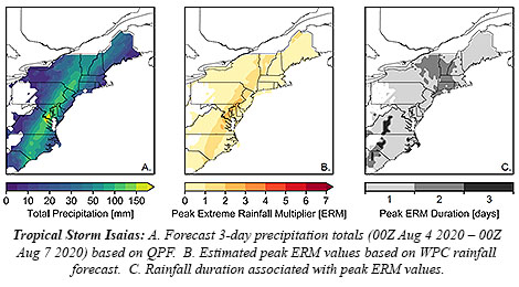
Tropical Storm Isaias is soaking the Mid-Atlantic states with what is expected to be three times as much rain as is typical for the area. Today’s heaviest tropical showers could trigger potentially deadly flash floods.
The projection is the finding of a new Intuitive Metric for Deadly Tropical Cyclone Rains, which we blogged about on The Front Page in June. The extreme rainfall multiplier (ERM) used the quantitative precipitation forecast (QPF) from the Storm Prediction Center last night to generate an ERM forecast for Isaias.
“Since Isaias is a fast-moving storm (currently moving NNE at 23 mph), the heaviest rain is forecast to fall with[in] a 24-hour period today (Aug 4)”, wrote the study’s lead author, Christopher Bosma, a Ph.D. student at the University of Wisconsin-Madison, in a-pre-dawn e-mail. “Peak rainfall totals are projected to be just over 6 inches (approx. 150 mm), mostly in a narrow region just south of the DC Metro [area].”
In contrast, the region’s heaviest single-day, 2-year rainfall event is a bit more than 50 mm. Bosma uses that comparison in generating an ERM around 2.86 (152 mm / 53 mm). Rainfall may exceed the projections, but that gives a rough idea of how the storm compares to others in residents’ recent memory.
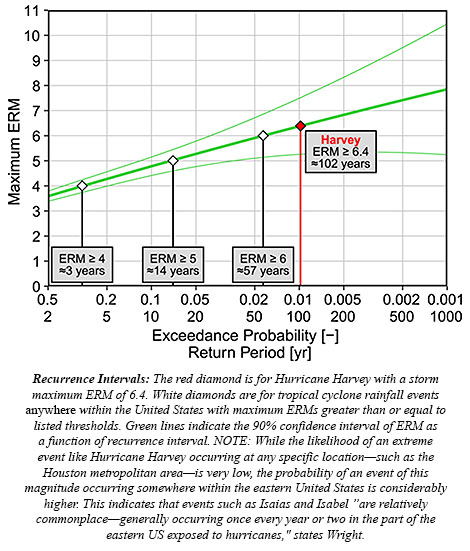
According to the study, which was published in the Bulletin of the American Meteorological Society in May, the average value of an ERM in U.S. landfalling hurricanes and tropical storms is 2.0. ERMs can hindcast the severity of precipitation for such storms, like 2017’s Hurricane Harvey. Harvey deluged Texas with as much as 60 inches of rain and reached an ERM of 6.4—the highest calculated.
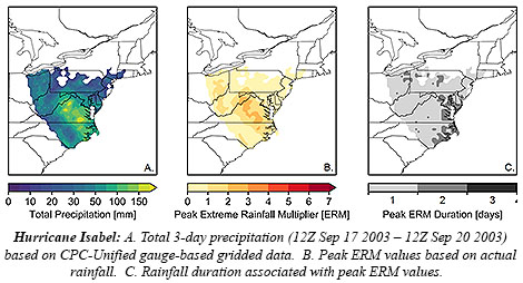
Those having lived in the D.C. area in the early 2000s might recall a tropical storm that Bosma says is comparable to Isaias: Isabel. After landfall in eastern North Carolina as a Cat. 2 hurricane the morning of September 18, 2003, it barreled north-northwest through the Mid-Atlantic delivering flooding rains and damaging winds that night.
“Isabel was also a fast mover at landfall, and was responsible for similar one-day rain totals of just over 6 inches, based on CPC-Unified gauge-based gridded data,” Bosma wrote.” The peak ERM for Isabel was 2.8. One thing to note from Isabel is that localized rainfall totals were higher in some spots, particularly in the mountains of Virginia, highlighting the threat of localized flash flooding that might also be present today with Isaias.”
Indeed, flash flood warnings were issued all across the interior Mid-Atlantic this morning. This was despite drought conditions in parts of the area.
Bosma and colleagues Daniel Wright (UW-Madison), J. Marshall Shepherd (University of Georgia), et al., created the ERM metric to focus on the deadly hazard of extreme tropical cyclone rainfall. Getting word out about the threat using only the wind-based Saffir-Simpson Scale “was a problem brought to light with Hurricanes Harvey and Florence,” Shepherd says.
Wright also in an e-mail last night stated that for Isaias in and around Washington, D.C., it’s “a fairly large amount of rain, though certainly not unprecedented for the region.”
 Last week’s derecho, roaring 750 miles from eastern Nebraska across Iowa, Illinois and Indiana, was particularly ferocious with winds in multiple swaths across Iowa gusting to over 100 mph. The National Weather Service found damage to an apartment complex in Cedar Rapids, Iowa, consistent with wind gusts of an astonishing 130-140 mph. But even these extreme winds and the severe damage they wrought don’t tell the whole story of the variation in these windy storms with the seemingly odd name.
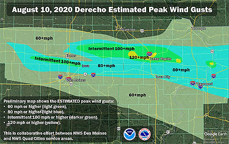 The AMS
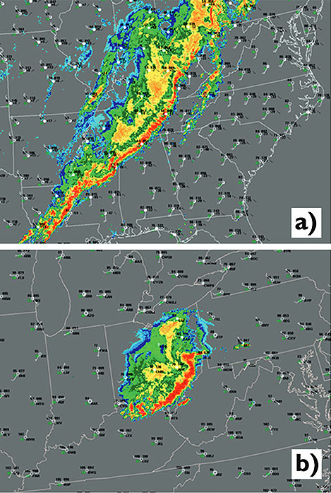
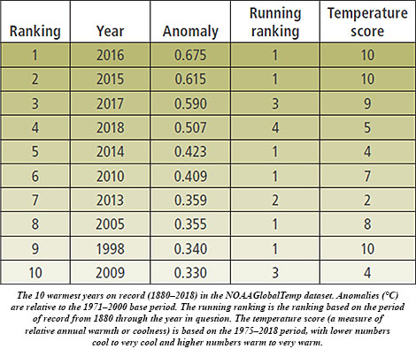 The temperature score from 1 (a very cold year) to 10 (very warm) is useful to distinguish between warmer and colder years relative to the long-term trend. As examples, the authors note that 2008 and 2011 were considerably cooler than surrounding years and below the overall trend, whereas 1998 and 2016 were not only the warmest years on record but were also notably warmer than surrounding years.
 BAMS: What would you like readers to learn from your study of record global temperatures?
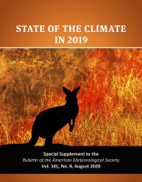 Despite the rapid pace of writing, editing, and reviewing, this is obviously not the first (or last) assessment of 2019’s climate. So we still often get asked—why now? Why release in August 2020 a comprehensive, validated check-up on the health of our planet’s climate in 2019 August, instead of in January, when it’s still hot news?
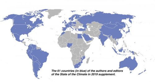 In just the past decade alone Blunden and Arndt have added 150 authors and 13 additional countries. Why so many authors?
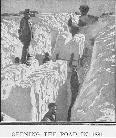 Boustead and co-authors Martha D. Shulski and Steven D. Hilberg set out to determine which parts of Laura’s stories are based in fact, and in the process, filled in the gap left by the absence of analysis or documentation in scientific literature about the Hard Winter of 1880-81. In the process, Boustead et al. show that the Hard Winter places recent severe winters, such as 2013-14, into context.
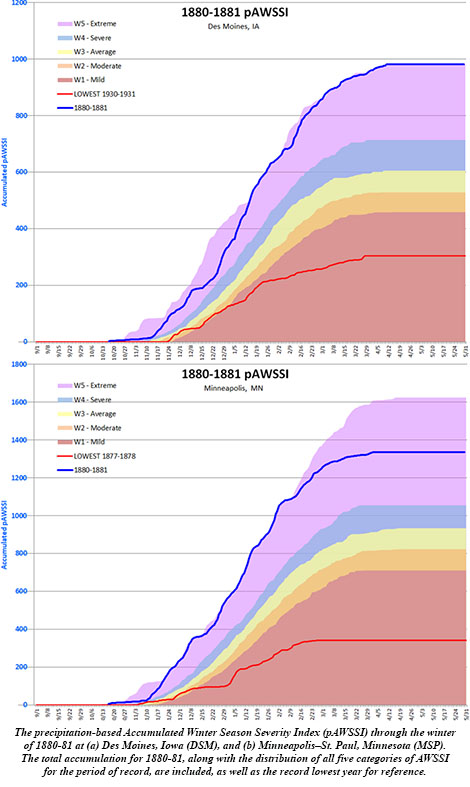 BAMS asked a few questions of Boustead to gain insight into her research. A sampling of answers are below:
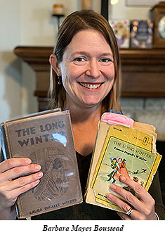 Barbara Mayes Boustead: The Long Winter research began over a decade ago as I reread the book as a “comfort read” on the tail end of a winter, reminding myself that even the longest winters do eventually end. I’ve been reading Laura Ingalls Wilder’s books since I was in elementary school, and I had always wondered if the winter was really as Wilder had described it. And then I got to thinking – I am a meteorologist, and I have the tools to look it up! The deeper I dug, the more that my questions led to more questions. I especially got excited as I found data that verified much of the weather that Wilder had described. And I knew I had found a resonant topic when I presented the work at a conference called LauraPalooza in 2010 (it’s real and it’s serious!) and was overwhelmed with questions and discussion following my presentation.
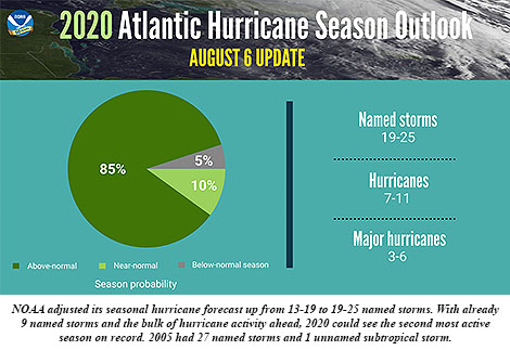 In that assessment of the current literature, Tom Knutson (NOAA) and other top tropical experts reviewed a number of peer-reviewed studies and determined that a majority found the numbers of named storms actually decrease in climate projections as we move deeper into this century. But there was no consensus among the authors to either support or refute those studies since their research also showed that “there is no clear observational evidence for a detectable human influence on historical global TC frequency.”