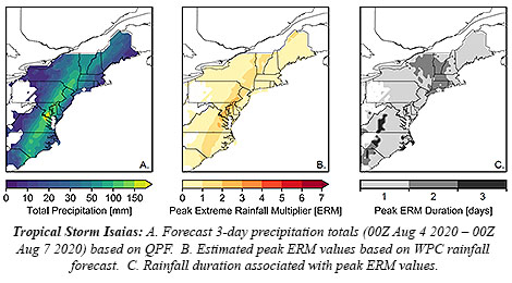
Tropical Storm Isaias is soaking the Mid-Atlantic states with what is expected to be three times as much rain as is typical for the area. Today’s heaviest tropical showers could trigger potentially deadly flash floods.
The projection is the finding of a new Intuitive Metric for Deadly Tropical Cyclone Rains, which we blogged about on The Front Page in June. The extreme rainfall multiplier (ERM) used the quantitative precipitation forecast (QPF) from the Storm Prediction Center last night to generate an ERM forecast for Isaias.
“Since Isaias is a fast-moving storm (currently moving NNE at 23 mph), the heaviest rain is forecast to fall with[in] a 24-hour period today (Aug 4)”, wrote the study’s lead author, Christopher Bosma, a Ph.D. student at the University of Wisconsin-Madison, in a-pre-dawn e-mail. “Peak rainfall totals are projected to be just over 6 inches (approx. 150 mm), mostly in a narrow region just south of the DC Metro [area].”
In contrast, the region’s heaviest single-day, 2-year rainfall event is a bit more than 50 mm. Bosma uses that comparison in generating an ERM around 2.86 (152 mm / 53 mm). Rainfall may exceed the projections, but that gives a rough idea of how the storm compares to others in residents’ recent memory.
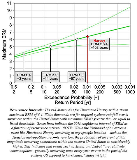
According to the study, which was published in the Bulletin of the American Meteorological Society in May, the average value of an ERM in U.S. landfalling hurricanes and tropical storms is 2.0. ERMs can hindcast the severity of precipitation for such storms, like 2017’s Hurricane Harvey. Harvey deluged Texas with as much as 60 inches of rain and reached an ERM of 6.4—the highest calculated.
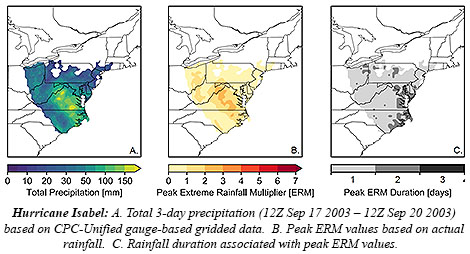
Those having lived in the D.C. area in the early 2000s might recall a tropical storm that Bosma says is comparable to Isaias: Isabel. After landfall in eastern North Carolina as a Cat. 2 hurricane the morning of September 18, 2003, it barreled north-northwest through the Mid-Atlantic delivering flooding rains and damaging winds that night.
“Isabel was also a fast mover at landfall, and was responsible for similar one-day rain totals of just over 6 inches, based on CPC-Unified gauge-based gridded data,” Bosma wrote.” The peak ERM for Isabel was 2.8. One thing to note from Isabel is that localized rainfall totals were higher in some spots, particularly in the mountains of Virginia, highlighting the threat of localized flash flooding that might also be present today with Isaias.”
Indeed, flash flood warnings were issued all across the interior Mid-Atlantic this morning. This was despite drought conditions in parts of the area.
Bosma and colleagues Daniel Wright (UW-Madison), J. Marshall Shepherd (University of Georgia), et al., created the ERM metric to focus on the deadly hazard of extreme tropical cyclone rainfall. Getting word out about the threat using only the wind-based Saffir-Simpson Scale “was a problem brought to light with Hurricanes Harvey and Florence,” Shepherd says.
Wright also in an e-mail last night stated that for Isaias in and around Washington, D.C., it’s “a fairly large amount of rain, though certainly not unprecedented for the region.”
Tropical Storm Isaias is soaking the Mid-Atlantic states with what is expected to be three times as much rain as is typical for the area. Today’s heaviest tropical showers could trigger potentially deadly flash floods.
The projection is the finding of a new Intuitive Metric for Deadly Tropical Cyclone Rains, which we blogged about on The Front Page in June. The extreme rainfall multiplier (ERM) used the quantitative precipitation forecast (QPF) from the Storm Prediction Center last night to generate an ERM forecast for Isaias.
“Since Isaias is a fast-moving storm (currently moving NNE at 23 mph), the heaviest rain is forecast to fall with[in] a 24-hour period today (Aug 4)”, wrote the study’s lead author, Christopher Bosma, a Ph.D. student at the University of Wisconsin-Madison, in a-pre-dawn e-mail. “Peak rainfall totals are projected to be just over 6 inches (approx. 150 mm), mostly in a narrow region just south of the DC Metro [area].”
In contrast, the region’s heaviest single-day, 2-year rainfall event is a bit more than 50 mm. Bosma uses that comparison in generating an ERM around 2.86 (152 mm / 53 mm). Rainfall may exceed the projections, but that gives a rough idea of how the storm compares to others in residents’ recent memory.
According to the study, which was published in the Bulletin of the American Meteorological Society in May, the average value of an ERM in U.S. landfalling hurricanes and tropical storms is 2.0. ERMs can hindcast the severity of precipitation for such storms, like 2017’s Hurricane Harvey. Harvey deluged Texas with as much as 60 inches of rain and reached an ERM of 6.4—the highest calculated.
Those having lived in the D.C. area in the early 2000s might recall a tropical storm that Bosma says is comparable to Isaias: Isabel. After landfall in eastern North Carolina as a Cat. 2 hurricane the morning of September 18, 2003, it barreled north-northwest through the Mid-Atlantic delivering flooding rains and damaging winds that night.
“Isabel was also a fast mover at landfall, and was responsible for similar one-day rain totals of just over 6 inches, based on CPC-Unified gauge-based gridded data,” Bosma wrote.” The peak ERM for Isabel was 2.8. One thing to note from Isabel is that localized rainfall totals were higher in some spots, particularly in the mountains of Virginia, highlighting the threat of localized flash flooding that might also be present today with Isaias.”
Indeed, flash flood warnings were issued all across the interior Mid-Atlantic this morning. This was despite drought conditions in parts of the area.
Bosma and colleagues Daniel Wright (UW-Madison), J. Marshall Shepherd (University of Georgia), et al., created the ERM metric to focus on the deadly hazard of extreme tropical cyclone rainfall. Getting word out about the threat using only the wind-based Saffir-Simpson Scale “was a problem brought to light with Hurricanes Harvey and Florence,” Shepherd says.
Wright also in an e-mail last night stated that for Isaias in and around Washington, D.C., it’s “a fairly large amount of rain, though certainly not unprecedented for the region.”
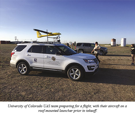
All the research ships and aircraft of atmospheric science may never be able to gather in one place for testing. But small, portable unmanned aircraft systems (UAS) are another matter. An international vanguard of scientists developing these atmospheric observing capabilities is finding that it is really helpful to get together to pool their insights—and devices—to accelerate each other’s progress. Together, their technology is taking off.
In the May 2020 BAMS, Gijs de Boer (CIRES and NOAA) and colleagues overview one of these coordinate-and-compare campaigns: when 10 teams from around the world brought 34 UAS to Colorado’s San Luis Valley for a week of tests, laying groundwork for new collaborations and future field programs. The July 2018 flight-fest conducted 1,300 research flights totaling more than 250 flight hours focused on observing the intricacies of the lower atmosphere.
At a “Community Day,” the scientists shared their aircraft and interests with the public as well. Working together all in one place has huge benefits. The teams get to see how they compare with each other, work out the kinks with their UAS, and move faster toward their research goals. It’s one reason they are getting so good so fast.
Below, de Boer answers some questions about the campaign and how he got started with UAS.
BAMS: What are some of the shared problems revealed by working together—as in LAPSE-RATE—with other UAS teams? Gijs de Boer: There are common problems at a variety of levels. For example, accurate wind sensing has proven challenging, and we’ve definitely worked together to improve wind estimation. Additionally, different modes of operation, understanding which sensors are good and which are not, and sensor placement are all examples of how the community has worked together to lift up the quality of measurements from all platforms.
BAMS: What are the most surprising lessons from LAPSE-RATE? GdB: I think that the continued rapid progression of the technology and the innovation in UAS-based atmospheric research is impressive. Some of the tools deployed during LAPSE-RATE in 2018 have already been significantly improved upon.
BAMS: What are some examples of this more recent UAS improvement? GdB: Everything continues to get smaller and lighter. Aircraft have become even more reliable, and instrumentation has continued to be scrutinized to improve data quality. Battery technology has also continued to improve, allowing for longer flight times and more complex missions.
Yet, we have so much more to do with respect to integrating our measurements into mainstream atmospheric research.
BAMS: What are some challenges to doing more to integrate UAS into research? GdB: Primarily, our UAV research community is working to demonstrate the reliability and accuracy of our measurements and platforms. This is critical to having them accepted in the community. There are also some other challenges associated with airspace access and development of infrastructure to interface these observations in both mainstream research and operations.
BAMS: It seems like there’s been success in this mainstreamed usage of UAS. GdB: Campaigns like LAPSE-RATE have paved the way for UAS to be more thoroughly included in larger field campaigns. A nice example is the recent ATOMIC (Atlantic Tradewind Ocean–Atmosphere Mesoscale Interaction Campaign) and EUREC4A (Elucidating the role of clouds-circulation coupling in climate) field campaigns, where three different UAS teams were involved and UAS were operated alongside manned research aircraft and in support of a much larger effort.
BAMS: How did you become interested in unmanned aviation? GdB: In 2011, I worked with a small group on a review article about our knowledge of mixed-phase clouds in Arctic environments. We took a good look at critical observational deficiencies, and I began to realize that many of the gaps involved a lack of in situ information, quantities that I thought could be measured by small platforms. This sent me down the road of investigating whether UAS could offer the necessary insight.
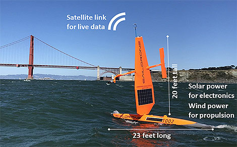
The Saildrone vehicle returning to San Francisco on June 11, 2018. The wind anemometer is visible at the top of the wing and solar panels are on both the wing and the vehicle hull. Image credit: Saildrone/Gentemann.
You’ve heard of drones in the air, but how about on the ocean’s surface? Enter Saildrone: A new wind and solar powered ocean-observing platform that carries a sophisticated suite of scientific sensors to observe air–sea fluxes. Looking like a large windsurfer without the surfer, the sailing drone glides autonomously at 2–8 kts. along the surface of uninhabited oceans on missions as long as 12 months, sampling key variables in the marine environment.
In a recent paper published in the Bulletin of the American Meteorological Society, author Chelle Gentemann and her colleagues explain that from April 11 to June 11, 2018, Saildrone cruised on a 60-day round trip from San Francisco down the coast to Mexico’s Guadelupe Island to establish the accuracy of its new measurements. These were made to validate air–sea fluxes, sea surface temperatures, and wind vectors derived by satellites. The automated surface vehicle also studied upwelling dynamics, river plumes, and the air–sea interactions of both frontal and diurnal warming regions on this deployment—meaning Saildrone’s versatile array of instruments got a workout not only above surface but just below it as well, in the water along the hull.
BAMS asked a few questions of the authors to gain insight into their research as well as their backgrounds. A sampling of answers are below:
Chelle Gentemann
BAMS: What would you like readers to learn from your article?
Chelle Gentemann, Farallon Institute: New measurement approaches are always being developed, allowing for new approaches to science. Understanding a dataset’s characteristics and uncertainties is important to have confidence in derived results.
BAMS: How did you become interested in working with Saildrone?
Gentemann: The ocean is a challenging environment to work in: it can be beautiful but dangerous, and gathering ship observations can require long absences from your family. I learned about Saildrones in 2016 and wanted to see how an autonomous vehicle might be able to gather data at the air–sea interface and adapt sampling to changing conditions. There are some questions that are hard to get at from existing remote sensing and in situ datasets; I thought that if these vehicles are able to collect high-quality data, they could be useful for science.
BAMS: How have you followed up on this experiment?
Gentemann: We sent two more [Saildrones] to the Arctic last Summer (2019) and are planning for two more in 2021. There are few in situ observations in the Arctic Ocean because of the seasonal ice cover, so sending Saildrones up there for the summer has allowed us to sample temperature and salinity fronts during a record heat wave.
Sebastien de Halleux, Saildrone, Inc.: I believe we are on the cusp of a new golden age in oceanography, as a wave of new enabling technologies is making planetary-scale in situ observations technically and economically feasible. The fact that Saildrones are zero-emission is a big bonus as we try to reduce our carbon footprint. I am excited to engage further with the science community to explore new ways of using this technology and developing tools to further the value of the data collected for the benefit of humanity.
BAMS: What got you initially interested in oceanography?
de Halleux:Having had the opportunity to sail across the Pacific several times, I developed a strong interest in learning more about the 70% of the planet covered by water—only to realize that the challenge of collecting data is formidable over such a vast domain. Being exposed to the amazing power of satellites to produce large-scale remote sensing datasets was only tempered by the realization of their challenges with fine features, land proximity, and of course the need to connect them to subsurface phenomena. This is how we began to explore the intersection of science, robotics, and big data with the goal to help enable new insights. Yet we are only at the beginning of an amazing journey.
BAMS:What surprises/surprised you the most about Saildrone’s capabilities?
Peter Minnett, Univ. of Miami, Florida: The ability to reprogram the vehicles in real time to focus on sampling and resampling interesting surface features. The quality of the measurements is impressive.
Saildrones are currently deployed around the world. In June 2019 , there were three circumnavigating Antarctica, six in the U.S. Arctic, seven surveying fish stock off the U.S. West Coast and two in Norway, four surveying the tropical Pacific, and one conducting a multibeam bathymetry survey in the Gulf of Mexico. In 2020, Saildrone, Inc. has deployed fleets in Europe, the Arctic, the tropical Pacific, along the West Coast, the Gulf of Mexico, the Atlantic, the Caribbean, and Antarctica. NOAA and NASA-funded Saildrone data are distributed openly and publicly.
The Saildrone vehicle returning to San Francisco on June 11, 2018. The wind anemometer is visible at the top of the wing and solar panels are on both the wing and the vehicle hull. Image credit: Saildrone/Gentemann.
You’ve heard of drones in the air, but how about on the ocean’s surface? Enter Saildrone: A new wind and solar powered ocean-observing platform that carries a sophisticated suite of scientific sensors to observe air–sea fluxes. Looking like a large windsurfer without the surfer, the sailing drone glides autonomously at 2–8 kts. along the surface of uninhabited oceans on missions as long as 12 months, sampling key variables in the marine environment.
In a recent paper published in the Bulletin of the American Meteorological Society, author Chelle Gentemann and her colleagues explain that from April 11 to June 11, 2018, Saildrone cruised on a 60-day round trip from San Francisco down the coast to Mexico’s Guadelupe Island to establish the accuracy of its new measurements. These were made to validate air–sea fluxes, sea surface temperatures, and wind vectors derived by satellites. The automated surface vehicle also studied upwelling dynamics, river plumes, and the air–sea interactions of both frontal and diurnal warming regions on this deployment—meaning Saildrone’s versatile array of instruments got a workout not only above surface but just below it as well, in the water along the hull.
BAMS asked a few questions of the authors to gain insight into their research as well as their backgrounds. A sampling of answers are below:
Chelle Gentemann
BAMS: What would you like readers to learn from your article?
Chelle Gentemann, Farallon Institute: New measurement approaches are always being developed, allowing for new approaches to science. Understanding a dataset’s characteristics and uncertainties is important to have confidence in derived results. BAMS: How did you become interested in working with Saildrone? Gentemann: The ocean is a challenging environment to work in: it can be beautiful but dangerous, and gathering ship observations can require long absences from your family. I learned about Saildrones in 2016 and wanted to see how an autonomous vehicle might be able to gather data at the air–sea interface and adapt sampling to changing conditions. There are some questions that are hard to get at from existing remote sensing and in situ datasets; I thought that if these vehicles are able to collect high-quality data, they could be useful for science. BAMS: How have you followed up on this experiment? Gentemann: We sent two more [Saildrones] to the Arctic last Summer (2019) and are planning for two more in 2021. There are few in situ observations in the Arctic Ocean because of the seasonal ice cover, so sending Saildrones up there for the summer has allowed us to sample temperature and salinity fronts during a record heat wave. Sebastien de Halleux, Saildrone, Inc.: I believe we are on the cusp of a new golden age in oceanography, as a wave of new enabling technologies is making planetary-scale in situ observations technically and economically feasible. The fact that Saildrones are zero-emission is a big bonus as we try to reduce our carbon footprint. I am excited to engage further with the science community to explore new ways of using this technology and developing tools to further the value of the data collected for the benefit of humanity. BAMS: What got you initially interested in oceanography? de Halleux:Having had the opportunity to sail across the Pacific several times, I developed a strong interest in learning more about the 70% of the planet covered by water—only to realize that the challenge of collecting data is formidable over such a vast domain. Being exposed to the amazing power of satellites to produce large-scale remote sensing datasets was only tempered by the realization of their challenges with fine features, land proximity, and of course the need to connect them to subsurface phenomena. This is how we began to explore the intersection of science, robotics, and big data with the goal to help enable new insights. Yet we are only at the beginning of an amazing journey. BAMS:What surprises/surprised you the most about Saildrone’s capabilities? Peter Minnett, Univ. of Miami, Florida: The ability to reprogram the vehicles in real time to focus on sampling and resampling interesting surface features. The quality of the measurements is impressive.
Saildrones are currently deployed around the world. In June 2019 , there were three circumnavigating Antarctica, six in the U.S. Arctic, seven surveying fish stock off the U.S. West Coast and two in Norway, four surveying the tropical Pacific, and one conducting a multibeam bathymetry survey in the Gulf of Mexico. In 2020, Saildrone, Inc. has deployed fleets in Europe, the Arctic, the tropical Pacific, along the West Coast, the Gulf of Mexico, the Atlantic, the Caribbean, and Antarctica. NOAA and NASA-funded Saildrone data are distributed openly and publicly.
Observations and models–that’s often an uneasy relationship. It’s not always easy to find the common ground needed to turn observations into model input and then models themselves into physically realistic output consistent with those observations.
DOE’s Atmospheric Radiation Measurement (ARM) program is trying to pull observing and modeling—ranging over vast time and space scales—tighter together, into effective bundles of science. Naturally, they’re using an initiative called “LASSO.”
Focused on shallow convection (often small, low-level scattered clouds), LASSO, or, the “Large-Eddy Simulation (LES) ARM Symbiotic Simulation and Observation” project centers on the capabilities of DOE’s Southern Plains observatory in Oklahoma. LASSO is designed to “add value to observations” through a carefully crafted modeling framework that evaluates how well the model “captures reality,” write William I. Gustafson and his colleagues in a paper recently published in the Bulletin of the American Meteorological Society (BAMS).
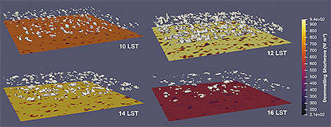
Renderings of cloud water isosurfaces (10−6 kg−1), every 2 h, show the diurnal evolution of a cloud field from a simulation forced by the VARANAL large-scale forcing on 30 Aug 2017. Cloud shadows can be seen in the surface downwelling shortwave radiation (colors; W m−2).
LASSO bundles data such as observations, LES input and output, and “quick-look” plots of the observations into a library of cases for study by modelers, theoreticians, and observationalists. LASSO includes diagnostics and skill scores of the extensive observations in the bundles and makes them freely available with simplified access for speedy use.
The goal of the data packaging approach is to enable scientists to more easily bridge the gap from smaller scale measurements and processes to the larger scale at which most modeling parameterizations operate.
We asked Gustafson to explain:
BAMS: What would you like readers to learn from this article?
Gustafson: In the atmospheric sciences we work with so many scales that we often get siloed into thinking in very scale-specific ways based on our sub-specialty and the type of research we do. This can happen whether we are modelers trying to wrap our brains around comparing parcel model simulations with global climate models, or as observationalists trying to rationalize differences between point-based surface measurements and big, pixel-based satellite measurements. The LASSO project is one attempt to get past limitations sometimes imposed by certain scales. For example, the DOE ARM program has such a wealth of measurements, and at the same time, DOE is developing a new and improved climate model. LASSO is one way to help marry the two together to add value for researchers working with both sets of data.
How did you become interested in the topic of this article?
My training is as a modeler, and over the years, a lot of my research has looked at issues of scale and how atmospheric models can better deal with unresolved detail—the so-called subgrid information. We know that subgrid information can be critical for properly simulating things like clouds and radiation. Yet, we cannot run global models with sufficient resolution to track this information. So, we need tools like large-eddy simulation to help us make better physics parameterizations for the coarser models used for weather prediction and climate change projections. Marrying the LES more tightly with observations seemed like a great way to help the atmospheric community move forward and make progress improving the models.
What got you initially interested in meteorology or the related field you are in?
I find weather fascinating and awe inspiring, and science has always been one of my interests alongside computers. Coming out of my undergrad years with a physics degree, I knew I wanted to pursue something related to computing, but I did not want to do it for a company for the sole purpose of making money for somebody. Atmospheric modeling seemed like a great way to apply my computer interests in an impactful way that would also be a lot of fun. Not many people get to play on giant supercomputers for a living trying to figure out what makes clouds do what they do. I have never looked back and much of my job I see as a grown-up playground where I get to build with computer bits instead of the sand I used to play with as a kid.
What surprises/surprised you the most about the work you document in this article?
This is not an article with filled with “ahah” moments. It is the result of years of effort put into developing a new data product that combines input from a large number of people with many different specialties. So, I would not say that I came across surprises.
However, I have come to really appreciate the help from so many people to make LASSO happen. We have people helping to collect input from dozens of instruments that have had to be maintained, data that has to be quality controlled, computers that are maintained, the actual modeling and packaging of the observations with the model output, the database and website development to make the product findable by users, the backhouse archive support, and communications specialists that have all been
critical to make LASSO happen.
What was the biggest challenge you encountered while doing this work?
Working with a long-term dataset has been one of our big challenges. We have been trying to put together a standardized data bundle that would make it easy for researchers to compare simulations from different cases spanning years. However, instrumentation changes from year to year, which means we continually have to adapt. Sometimes this presents itself as a new opportunity because of a new capability, such as a new photogrammetric cloud fraction product we are starting to work with. Other
times, existing instruments malfunction or are replaced with instruments that do not have the same capabilities, such as a switch from a two-channel to a three-channel microwave radiometer. The latter, in theory, could offer improved results, but in reality, led to years of calibration issues.
What’s next? How will you follow up?
The LASSO activity has been well received and we are excited to be expanding to new weather regimes. During 2020 we have been developing a new LASSO scenario that focuses on deep convection in Argentina. This is really exciting because storms in this area are some of the tallest in the world. It will also be a lot of fun working with LES of deep convection with all its associated cloud motions and detail. We plan to have this new scenario ready for release in 2021.
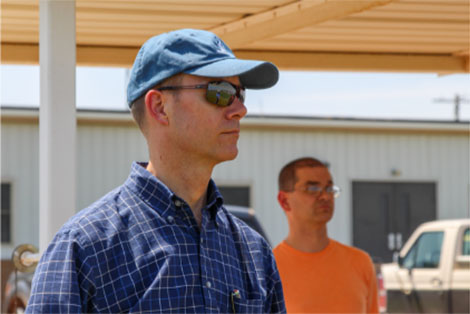
William Gustafson visited the DOE ARM’s Southern Great Plains Central Facility in 2016 near the beginning of the LASSO activity. Seeing the locations of the instruments within their natural environment has really helped put them into context and use them in conjunction with the LASSO LES modeling.
Observations and models–that’s often an uneasy relationship. It’s not always easy to find the common ground needed to turn observations into model input and then models themselves into physically realistic output consistent with those observations.
DOE’s Atmospheric Radiation Measurement (ARM) program is trying to pull observing and modeling—ranging over vast time and space scales—tighter together, into effective bundles of science. Naturally, they’re using an initiative called “LASSO.”
Focused on shallow convection (often small, low-level scattered clouds), LASSO, or, the “Large-Eddy Simulation (LES) ARM Symbiotic Simulation and Observation” project centers on the capabilities of DOE’s Southern Plains observatory in Oklahoma. LASSO is designed to “add value to observations” through a carefully crafted modeling framework that evaluates how well the model “captures reality,” write William I. Gustafson and his colleagues in a paper recently published in the Bulletin of the American Meteorological Society (BAMS).
Renderings of cloud water isosurfaces (10−6 kg−1), every 2 h, show the diurnal evolution of a cloud field from a simulation forced by the VARANAL large-scale forcing on 30 Aug 2017. Cloud shadows can be seen in the surface downwelling shortwave radiation (colors; W m−2).
LASSO bundles data such as observations, LES input and output, and “quick-look” plots of the observations into a library of cases for study by modelers, theoreticians, and observationalists. LASSO includes diagnostics and skill scores of the extensive observations in the bundles and makes them freely available with simplified access for speedy use.
The goal of the data packaging approach is to enable scientists to more easily bridge the gap from smaller scale measurements and processes to the larger scale at which most modeling parameterizations operate.
We asked Gustafson to explain: BAMS: What would you like readers to learn from this article? Gustafson: In the atmospheric sciences we work with so many scales that we often get siloed into thinking in very scale-specific ways based on our sub-specialty and the type of research we do. This can happen whether we are modelers trying to wrap our brains around comparing parcel model simulations with global climate models, or as observationalists trying to rationalize differences between point-based surface measurements and big, pixel-based satellite measurements. The LASSO project is one attempt to get past limitations sometimes imposed by certain scales. For example, the DOE ARM program has such a wealth of measurements, and at the same time, DOE is developing a new and improved climate model. LASSO is one way to help marry the two together to add value for researchers working with both sets of data. How did you become interested in the topic of this article?
My training is as a modeler, and over the years, a lot of my research has looked at issues of scale and how atmospheric models can better deal with unresolved detail—the so-called subgrid information. We know that subgrid information can be critical for properly simulating things like clouds and radiation. Yet, we cannot run global models with sufficient resolution to track this information. So, we need tools like large-eddy simulation to help us make better physics parameterizations for the coarser models used for weather prediction and climate change projections. Marrying the LES more tightly with observations seemed like a great way to help the atmospheric community move forward and make progress improving the models. What got you initially interested in meteorology or the related field you are in?
I find weather fascinating and awe inspiring, and science has always been one of my interests alongside computers. Coming out of my undergrad years with a physics degree, I knew I wanted to pursue something related to computing, but I did not want to do it for a company for the sole purpose of making money for somebody. Atmospheric modeling seemed like a great way to apply my computer interests in an impactful way that would also be a lot of fun. Not many people get to play on giant supercomputers for a living trying to figure out what makes clouds do what they do. I have never looked back and much of my job I see as a grown-up playground where I get to build with computer bits instead of the sand I used to play with as a kid. What surprises/surprised you the most about the work you document in this article?
This is not an article with filled with “ahah” moments. It is the result of years of effort put into developing a new data product that combines input from a large number of people with many different specialties. So, I would not say that I came across surprises.
However, I have come to really appreciate the help from so many people to make LASSO happen. We have people helping to collect input from dozens of instruments that have had to be maintained, data that has to be quality controlled, computers that are maintained, the actual modeling and packaging of the observations with the model output, the database and website development to make the product findable by users, the backhouse archive support, and communications specialists that have all been
critical to make LASSO happen. What was the biggest challenge you encountered while doing this work?
Working with a long-term dataset has been one of our big challenges. We have been trying to put together a standardized data bundle that would make it easy for researchers to compare simulations from different cases spanning years. However, instrumentation changes from year to year, which means we continually have to adapt. Sometimes this presents itself as a new opportunity because of a new capability, such as a new photogrammetric cloud fraction product we are starting to work with. Other
times, existing instruments malfunction or are replaced with instruments that do not have the same capabilities, such as a switch from a two-channel to a three-channel microwave radiometer. The latter, in theory, could offer improved results, but in reality, led to years of calibration issues. What’s next? How will you follow up?
The LASSO activity has been well received and we are excited to be expanding to new weather regimes. During 2020 we have been developing a new LASSO scenario that focuses on deep convection in Argentina. This is really exciting because storms in this area are some of the tallest in the world. It will also be a lot of fun working with LES of deep convection with all its associated cloud motions and detail. We plan to have this new scenario ready for release in 2021.
William Gustafson visited the DOE ARM’s Southern Great Plains Central Facility in 2016 near the beginning of the LASSO activity. Seeing the locations of the instruments within their natural environment has really helped put them into context and use them in conjunction with the LASSO LES modeling.
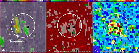
Many of us will not be seeing fireworks this Independence Day, due to coronavirus restrictions and local ordinances. But one way to make up for not seeing festive explosions of color and fire in person this year might be to see what they look like…on weather radar.
Willow fireworks 2.3 s after burst. The three smaller bursts are at earlier stages of development. The one in the upper-right corner is at 270 m above ground, the highest of the bursts in the study.
In “Fireworks on Weather Radar and Camera,” published recently in the Bulletin of the AMS (BAMS), Dusan Zrnic (National Severe Storms Laboratory) and his colleagues looked at Fourth of July fireworks in Norman, Oklahoma, and Fort Worth, Texas, using reflectivity data and the dual-pol capability on finer resolution radar, which could discern meteor sizes from the explosions.
The three types of radars were: NSSL’s research (3-cm wavelength) dual-polarization radar, the Terminal Doppler Weather Radar (TDWR) that operates in single polarization at a 5-cm wavelength from the Oklahoma City airport, and NWS Doppler radar in both Norman and Fort Worth. To complement the radar, video was taken of the shows.
In Norman, they found bursts were typically 100 to 200 m above ground and a few of them spread to 200 m in diameter. Some of the meteors fell at 22 m s-1, or about the fall speed of large hail. The Fort Worth fireworks were often much larger, and reflectivity could cover an area about 800 m to more than 2,000 m across–four times as big as in Norman. The peak reflectivity signals in Fort Worth were also greater.
Fields of reflectivity Z (in dBZ), Doppler velocity υr (in m s−1), and Doppler spectrum width συ (in m s−1). The diameter of the white circle is 3.5 km. The data are from the operational WSR-88D over the Dallas–Fort Worth metro area. The arrow points to the patch caused by the fireworks. The patch to the right is caused by reflections off buildings.
In polarimetric radar views of the Norman fireworks, the pyrotechnics signals blended with those from living things like insects, birds or bats. In the Fort Worth case, the backscatter differential phase and the differential reflectivity were in the range of giant hail.
We asked Dr. Zrnic to help us understand his motivations for this work.
How did you get started in observational studies with weather radar?
I have a degree in electrical engineering and was interested in applying my knowledge of random signals to useful purposes. I received a postdoctoral position at the National Severe Storms Laboratory, where in 1973 they had collected data from a violent tornado in Union City, Oklahoma, to gauge its maximum rotational speed. It was about 15 years ahead of any similar collection elsewhere. Upon my arrival I was given the opportunity to work on determining the Doppler spectra of the tornado. That was how I ended up comparing simulated to observed spectra. We observed a reflectivity maximum at a certain radial distance—a “doughnut” type profile that we posited was caused by drops with size and rotational speed for which the centrifugal and centripetal forces were in equilibrium. The rest is history.
What would you like readers to learn from this article?
Operational, polarimetric radars detect fireworks. Also, by comparing reflectivity at three wavelengths we can roughly estimate the dominant size of “stars” of fireworks.
Was this a surprise?
We expected that the polarimetric variables would detect the bursts, but we were surprised by the high values of reflectivities: 47 dBZ from large metropolitan displays versus 39 dBZ for small municipal fireworks as in Norman. These high reflectivity values can bias rainfall measurements unless they are eliminated from further processing.
Why study fireworks on radar?
Initially we were trying to identify onsets and locations of fires and explosions. We found we could do this using historic WSR-88D data, but not very well. Then my co-author Valery Melnikov suggested that fireworks could be a proxy for these events and this turned out to be true. The obvious advantage is that the exact place and time of fireworks detonation is known, making it is easy to locate a mobile radar in a favorable position to obtain key data.
What else surprised you?
The highest fall speeds of about 22 m s-1 exceeded our expectations. We also did not realize how transient the returns are; a firework can be seen by eye for up to several seconds and after that it turns into ash, which is not detectable by radar.
What was the biggest challenge you encountered?
We were hoping we might be able to observe the dispersion of Doppler velocities in the Doppler spectra and collected such data. Unfortunately, we lost these data. Another first for us was to learn how to use software for displaying visual images; once we learned, it became a matter of time to do the analysis. Also, to develop the backscattering model of “stars” required extensive literature search. There is no information about the refractive index of “stars” so we had to look up the composition of these and estimate the values for mixtures of three ingredients. The good thing is that the results are not very sensitive to a range of possible values.
Fireworks on radar may be quieter, but the paper shows that—on polarimentric displays—they’re just as colorful. When your local fireworks shows finally return, the authors advise, “using smart phones, the public can observe radar images and the real thing at the same time.”
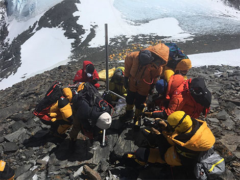
An automatic weather station (AWS) being installed on Everest’s South Col at 7,945 m (~26,066 ft). Note the tents of Camp IV in the background, and the exposed glacier ice visible behind. [Photo credit: Baker Perry / National Geographic.]
Despite freezing temperatures, snow is melting on Mount Everest. That’s just one finding in a recent study of weather data provided by a new network of five automated weather stations on Earth’s tallest mountain. The network includes two of the highest altitude weather stations on Earth, Balcony Station at 8,430 m (~27,658 ft) and South Col at 7,945 m (~26,066 ft), and offers “an unrivaled natural platform for measuring ongoing climate change across the full elevation range of Asia’s water towers,” Tom Matthews and his colleagues write in their new article published as an Early Online Release in the Bulletin of the American Meteorological Society.
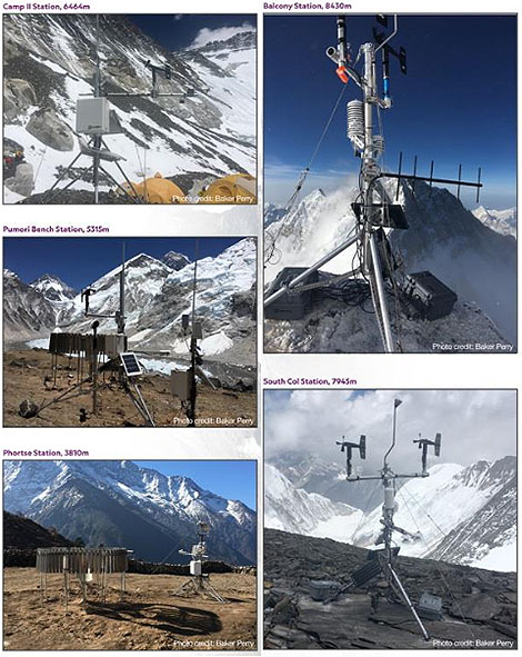
Photos of the automatic weather stations installed during the 2019 Everest Expedition. Note the shovel handles used to mount the wind speed sensors on the Balcony weather station (upper right).
The snowmelt is attributed to extreme insolation in the high altitudes of the Himalaya. It enables “considerable” melt up to Camp II at an altitude of 6,464 m (~21,207 ft), “despite freezing air temperatures,” the study reports. And modeling with the data the five stations are providing shows not only is melting occurring at South Col even with average air temperatures of -10°C—which means melting may be common at the tops of all but a small portion of the peaks in the Himalaya—but also is likely happening even at Everest’s peak, Matthews and his team report.
Uncertainties in the extrapolation are considerable, but we cannot rule out that limited melting during the monsoon may be occurring at the summit.
The authors note that while snow melting at the peak of the world’s tallest mountain may be “symbolic” as Earth continues to warm, sublimation of the snowpack appears to be a far greater contributor to its loss at such high altitudes. This finding has implications for the amount of snow that actually falls at extreme altitudes:
The amount of mass potentially lost by sublimation on the upper slopes of Everest, coupled with the presence of permanent snow cover over much of this terrain, raises the interesting prospect that snowfall at such altitudes in the Himalaya may be more substantial than previously thought. For example, the modeled sublimation of 128 mm at the South Col (in five months) is almost eight times greater than the predicted annual precipitation at such altitude. Windblown snow from lower elevations may account for much of the discrepancy, but the winds are also known to deflate the snow on Everest, sometimes to spectacular effect. Future work is clearly needed to rule out the possibility of a much more vigorous hydrological cycle at these extreme elevations.
Matthews and his coauthors conclude that the data the five AWSs have collected so far offer “rich opportunities” to adjust and improve mountain weather forecasting and melt modeling.
Uncontrollable sources of ozone from stratospheric intrusions, wildfires, and intercontinental transport are complicating efforts in California to further reduce this pollutant, which is particularly harmful to our health.
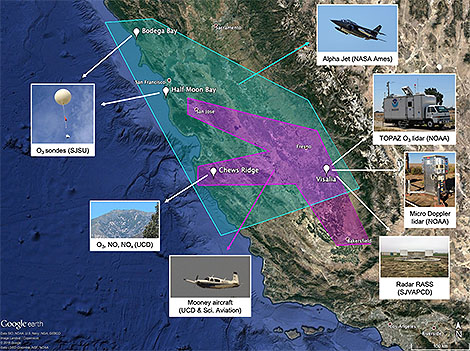
Scientists measured daily fluctuations in ozone in the air across Northern and Central California in 2016 during a coordinated field campaign known as the California Baseline Ozone Transport Study. They particularly focused on ozone crossing the shoreline and accumulating in low level air over the San Joaquin Valley.
Ian Faloona (University of California, Davis) and colleagues summarize the measurements and unique meteorological context for this novel dataset in a recent article published in the Bulletin of the American Meteorological Society. Faloona et al. draw attention to the dataset’s potential for future modeling studies of the impacts of long-range transport on regional air quality.
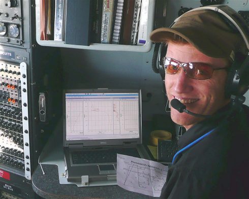
Falloona, in his cockpit perch during aerial measurements for CABOTS.
We asked lead author Faloona to help us understand CABOTS and his motivations for this work.
BAMS: What would you like readers to learn from this article?
Faloona: I think this article presents a nice overview of the mesoscale flow over the complex terrain of Central and Northern California, and I would like readers to become more appreciative of the global nature of air pollution. The field of air quality was once considered in terms of emissions and receptors within “air basins” but as our knowledge of the global nature of greenhouse gases in terms of climate change has developed, I believe that we have similarly become more and more aware of the global aspects of many air pollutants in general.
The CABOTS study domain and measurement platforms ranged from daily ozonesondes launched at the two coastal sites (Bodega Bay and Half Moon Bay) to the NOAA TOPAZ lidar in Visalia. The green and purple polygons represent the approximate domains surveyed by the NASA Alpha jet and Scientific Aviation, Inc., Mooney air-craft, respectively.
How did you become interested in the topic of this article?
Some colleagues from the UC Davis Air Quality Research Center and I became interested in long-range transport of air pollution to California and how it might be best sampled along the coastal mountains where local emissions might be minimal and the surface was well above the strong temperature inversion of the marine boundary layer. We eventually found the site on Chews Ridge where a group of renegade astronomers had been operating an off-the-grid observatory with the Monterey Institute for Research in Astronomy. They allowed us to build a climate monitoring site collocated with their observatory (the Oliver Observing Station) and then some airborne work for the San Joaquin Valley Air Pollution Control District allowed us to link the inflow at the coast to air quality issues within the leeward valley.
What got you initially interested in meteorology or in the related field you are in?
While an undergraduate studying physical chemistry I wrote a term paper on acid rain for a chemical oceanography class. I was floored by how few details were thoroughly understood about the chemical mechanisms of an environmental problem that at the time was considered quite serious. I figured I should throw whatever brainpower heft I could into this type of atmospheric oxidation chemistry. But then, while working for a private consulting company in Colorado after college, many of my colleagues there were trained in meteorology and I knew there would be little progress without a fundamental understanding that field. So I went to Penn State to do chemistry research but get trained in all aspects of meteorology.
What surprises/surprised you the most about the work you document in this article?
The first thing that surprised me about the data we collected for CABOTS was how deep the daytime up-valley flow was (~1.5 km), but how shallow the convective boundary layers tended to be (~0.5 km). The scale interactions that need to be taken into account when analyzing boundary layers among the complex terrain of California make it a great place to study in meteorology. But the other major discovery that came out of this work was the evidence we found of significant NOx emissions from certain agricultural regions in the San Joaquin Valley. For instance, we found that the agricultural region between Fresno and Visalia was responsible for as much NOx emitted to the valley atmosphere as from all the mobile sources in the CARB inventory across the three county region.
What was the biggest challenge you encountered while doing this work?
The sensible heat at the Fresno airport. Our airborne deployments attempted to target high ozone episodes, which are best forecast by their correlation with ambient temperatures. I like to tell my students that I am a chaser of extreme weather. It just so happens that the weather features most important to air quality are heat waves. Heat waves are extremely easy to catch, and can be brutal in their persistence. Some days we observed temperatures in the plane on the tarmac of >115 ºF, which made it challenging to keep the equipment up and running. I remember dragging bags of ice in and out of the plane covered in sweat, and still having the instruments give up in heat exhaustion before one of our midday flights.
What’s next? How will you follow up?
I would like to continue studying the various scales at play in the transport of intercontinental pollution to North America, and my preferred tools are aircraft laboratories. I would like to follow up with a study of wintertime stagnation events that lead to particulate matter air quality problems – an entirely different meteorological beast. But I would also like to follow up with a study of agricultural NOx emissions in the Imperial Valley of Southern California. This region is expected to have the largest soil emissions and the lowest urban sources to confound the measurements. It is also a region of important environmental justice issues being made up largely of migrant agricultural workers who have to bear the burden of the air quality problems engendered by agriculture.
 At a “Community Day,” the scientists shared their aircraft and interests with the public as well. Working together all in one place has huge benefits. The teams get to see how they compare with each other, work out the kinks with their UAS, and move faster toward their research goals. It’s one reason they are getting so good so fast.