The Thanksgiving holiday weekend has long been heralded as the start of the Western United States winter ski season. But new research using regional climate models sees Thanksgiving skiing going cold turkey.
As climate change ramps up into the mid twenty-first century, we can expect shorter ski seasons from the Southwest to the northern Rockies. This includes projections for less snow as well as poorer conditions for artificial snowmaking in the mountain states of the interior West. These are the findings from new research presented by Christian Lackner (Univ. of Wyoming and Johannes Gutenberg-Univ. of Mainz) this week at the American Meteorological Society’s 19th Conference on Mountain Meteorology. Despite being entirely on-line, the meeting achieved record attendance.
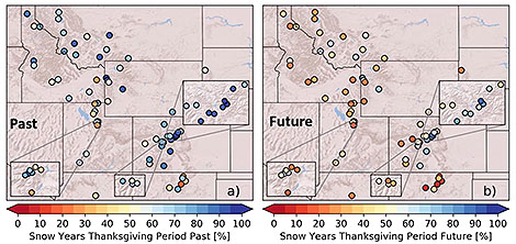
Lackner’s presentation, co-authored with Bart Geerts and Yonggang Wang, showed that the downturn in the ski season is projected to impact lower-elevation ski areas such as those in Arizona and New Mexico the most. Ski seasons by 2050 will start about two weeks later and end two-to-three weeks earlier than in the baseline period of 1981-2010. For many resorts that means the season length is seen to fall below the 100-day threshold long viewed as the make-it-or-break point for staying viable in the ski industry.
Higher-elevation ski resorts in Colorado, Utah, and western Wyoming, as well as higher latitude ski areas in Montana and Idaho, will fair better, although they’ll see their seasons shrink by 10-20 days. That will drop them below 120 days—the high-elevation, high-latitude resorts’ economic threshold—by 2050.
Lackner et al.’s study looked at climate change impacts at 71 ski resorts in Arizona, Colorado, Idaho, Montana, New Mexico, and Wyoming from November 15-April 15, the key cold-season months.
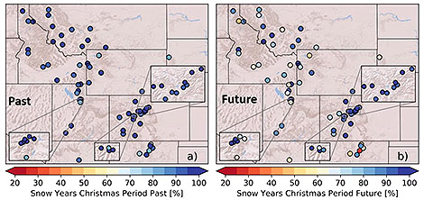
The good news is the Christmas holiday week still looks good for shooshing down Western slopes, despite the climate projections.
 amsblog_2nx4m1
"LASSO" It for Science
Observations and models–that’s often an uneasy relationship. It’s not always easy to find the common ground needed to turn observations into model input and then models themselves into physically realistic output consistent with those observations.
DOE’s Atmospheric Radiation Measurement (ARM) program is trying to pull observing and modeling—ranging over vast time and space scales—tighter together, into effective bundles of science. Naturally, they’re using an initiative called “LASSO.”
Focused on shallow convection (often small, low-level scattered clouds), LASSO, or, the “Large-Eddy Simulation (LES) ARM Symbiotic Simulation and Observation” project centers on the capabilities of DOE’s Southern Plains observatory in Oklahoma. LASSO is designed to “add value to observations” through a carefully crafted modeling framework that evaluates how well the model “captures reality,” write William I. Gustafson and his colleagues in a paper recently published in the Bulletin of the American Meteorological Society (BAMS).
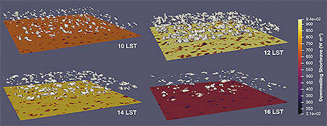
LASSO bundles data such as observations, LES input and output, and “quick-look” plots of the observations into a library of cases for study by modelers, theoreticians, and observationalists. LASSO includes diagnostics and skill scores of the extensive observations in the bundles and makes them freely available with simplified access for speedy use.
The goal of the data packaging approach is to enable scientists to more easily bridge the gap from smaller scale measurements and processes to the larger scale at which most modeling parameterizations operate.
We asked Gustafson to explain:
BAMS: What would you like readers to learn from this article?
Gustafson: In the atmospheric sciences we work with so many scales that we often get siloed into thinking in very scale-specific ways based on our sub-specialty and the type of research we do. This can happen whether we are modelers trying to wrap our brains around comparing parcel model simulations with global climate models, or as observationalists trying to rationalize differences between point-based surface measurements and big, pixel-based satellite measurements. The LASSO project is one attempt to get past limitations sometimes imposed by certain scales. For example, the DOE ARM program has such a wealth of measurements, and at the same time, DOE is developing a new and improved climate model. LASSO is one way to help marry the two together to add value for researchers working with both sets of data.
How did you become interested in the topic of this article?
My training is as a modeler, and over the years, a lot of my research has looked at issues of scale and how atmospheric models can better deal with unresolved detail—the so-called subgrid information. We know that subgrid information can be critical for properly simulating things like clouds and radiation. Yet, we cannot run global models with sufficient resolution to track this information. So, we need tools like large-eddy simulation to help us make better physics parameterizations for the coarser models used for weather prediction and climate change projections. Marrying the LES more tightly with observations seemed like a great way to help the atmospheric community move forward and make progress improving the models.
What got you initially interested in meteorology or the related field you are in?
I find weather fascinating and awe inspiring, and science has always been one of my interests alongside computers. Coming out of my undergrad years with a physics degree, I knew I wanted to pursue something related to computing, but I did not want to do it for a company for the sole purpose of making money for somebody. Atmospheric modeling seemed like a great way to apply my computer interests in an impactful way that would also be a lot of fun. Not many people get to play on giant supercomputers for a living trying to figure out what makes clouds do what they do. I have never looked back and much of my job I see as a grown-up playground where I get to build with computer bits instead of the sand I used to play with as a kid.
What surprises/surprised you the most about the work you document in this article?
This is not an article with filled with “ahah” moments. It is the result of years of effort put into developing a new data product that combines input from a large number of people with many different specialties. So, I would not say that I came across surprises.
However, I have come to really appreciate the help from so many people to make LASSO happen. We have people helping to collect input from dozens of instruments that have had to be maintained, data that has to be quality controlled, computers that are maintained, the actual modeling and packaging of the observations with the model output, the database and website development to make the product findable by users, the backhouse archive support, and communications specialists that have all been
critical to make LASSO happen.
What was the biggest challenge you encountered while doing this work?
Working with a long-term dataset has been one of our big challenges. We have been trying to put together a standardized data bundle that would make it easy for researchers to compare simulations from different cases spanning years. However, instrumentation changes from year to year, which means we continually have to adapt. Sometimes this presents itself as a new opportunity because of a new capability, such as a new photogrammetric cloud fraction product we are starting to work with. Other
times, existing instruments malfunction or are replaced with instruments that do not have the same capabilities, such as a switch from a two-channel to a three-channel microwave radiometer. The latter, in theory, could offer improved results, but in reality, led to years of calibration issues.
What’s next? How will you follow up?
The LASSO activity has been well received and we are excited to be expanding to new weather regimes. During 2020 we have been developing a new LASSO scenario that focuses on deep convection in Argentina. This is really exciting because storms in this area are some of the tallest in the world. It will also be a lot of fun working with LES of deep convection with all its associated cloud motions and detail. We plan to have this new scenario ready for release in 2021.
"Decision-making under meteorological uncertainty" for D-Day's Famous Forecast
The success of the D-Day Invasion of Normandy was due in part to one of history’s most famous weather forecasts, but new research shows this scientific success resulted more from luck than skill. Oft-neglected historical documentation, including audio files of top-secret phone calls, shows the forecasters were experiencing a situation still researched and practiced today: “decision-making under meteorological uncertainty.”
New research recently published in BAMS into that weather forecast for June 6, 1944, which enabled the Allies in World War II to gain a foothold in Europe, answers questions about three popular perceptions: were the forecasts, which predicted a break in the weather, that good? were the German meteorologists so ill-informed, missing that weather-break? and was the American analog system for prediction so great and better than what the Germans had?
The “alleged” weather break
An expected ridge and fair weather between two areas of low pressure, one departing and one arriving over the area, didn’t materialize. The departing low instead lingered and created a lull in visibility and lifted the cloud ceiling height, but it didn’t slow winds much. They blew at Force 4-5 (~13-24 mph), creating very choppy seas that sickened many troops prior to the invasion.
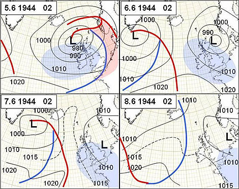
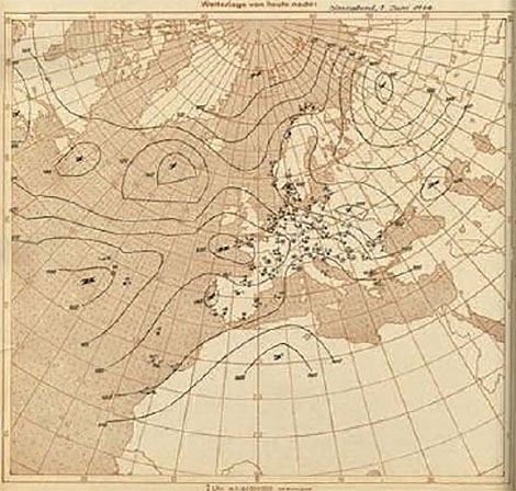
A blown German Forecast?
Because the invasion came as a complete surprise to the Germans it has been surmised their weather forecast for June 6 had to be bad. German forecasters prior to the war were the best at “extended” forecasts, and their synoptic maps and forecast for that day were more realistic than the Allies, with a less optimistic speculation of any break in the weather.
A historically debated forecast
The analog weather prediction system employed by the Allies for the invasion was claimed by its creators to have correctly identified the weather break. But historical analysis and review doesn’t bear this out. What it does find, though, is that the system correctly identified a transition from zonal to meridional flow, which delivered the break the Allies needed for success. History’s finding: The forecast was “Overoptimistic.”
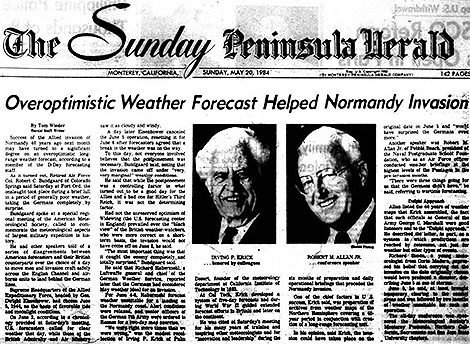
As a lesson learned from this most famous of weather forecasts, the paper’s author, Anders Persson of Swedin’s Uppsala University, concludes:
It was 75[+] years ago and the observational coverage has improved tremendously since then, both qualitatively and quantitatively. Our understanding of the atmosphere is much better,and the forecast methods have reached a standard that could hardly have been dreamt of in 1944. However, there’s one element that has a familiar ring to it and is of great interest today. That is when Air Marshall Tedder [Deputy Supreme Commander of the Invasion under General Eisenhower] asks about an assessment of the confidence in the forecast he has just heard … This illustrates that the D-day forecast is a significant early example of decision-making under meteorological uncertainty.
AMS's New Culture and Inclusion Cabinet
by Keith L. Seitter, CCM, AMS Executive Director
One of the AMS Core Values is: “We believe that a diverse, inclusive, and respectful community is essential for our science.”
AMS lives this value, which is articulated in the Centennial Update to the AMS Strategic Goals. We work to foster a culture that celebrates our diversity, strives for equity in all we do, and encourages inclusion across all activities so that everyone can experience a sense of belonging in the Society.
To formalize these efforts and provide a clearer path for providing resources toward them, the Council approved the creation of a new entity in AMS in fall 2019. At its meeting this past January, the Council approved the terms of reference for this new component of the Society’s structure and that Dr. Melissa Burt would serve as its first chair. This Culture and Inclusion Cabinet (CIC) has the following charge:
To accelerate the integration of a culture of inclusion, belonging, diversity, equity, and accessibility across the AMS and evaluate and assess progress towards culture and inclusion strategic goals within the Society. Meaningful integration into all areas and components of the AMS will require time and sustained effort. Fully integrating diversity, equity, inclusion, and belonging (DEIB) will result in an organizational culture that is accessible, advances science, serves society, and is responsive to social justice.
The Council designates this new body as a “Cabinet” to reinforce that it is not quite like any of the other entities making up the volunteer structure of the Society (council, commission, board, committee, task force, etc.). The CIC will play a unique role and therefore was given a unique name.
The CIC sits at the highest level of the organizational structure for AMS save the Council itself, to which it reports directly. Being at this level it can more readily ensure that issues of diversity, equity, inclusion, accessibility, social justice, and belonging are addressed throughout all AMS programs and activities.
The CIC does not replace any of the other components of the Society that work in these arenas—most notably the Board on Women and Minorities (BWM), which has a long record of addressing equity and inclusion issues in AMS. The BWM will continue to oversee specific programs aimed at diversity, equity, and inclusion, and will likely expand its role in AMS programs as the CIC helps integrate those efforts more broadly in the Society.
AMS has a strong record of addressing diversity and equity issues and a culture of inclusivity that other organizations could learn from. The creation of the CIC builds on those strengths and puts AMS in a position of leadership among scientific organizations in elevating these issues to the highest levels so that they can be threaded through every program in foundational ways.
For many of us, the sense of belonging in AMS is an important part of what makes the Society so special, and we want everyone in the community to feel that sense of belonging as an intrinsic aspect of the AMS culture. I am confident the new Culture and Inclusion Cabinet will take us there and will assist our entire community in creating an even more inclusive environment—strengthening our enterprise in the process.
Observations without Fear: NOAA's Drones for Hurricane Hunting
Nowhere is it more dangerous to fly in a hurricane than right near the roiling surface of the ocean. These days, hurricane hunting aircraft wisely steer clear of this boundary layer, but as a result observations at the bottom of the atmosphere where we experience storms are scarce. Enter the one kind of plane that’s fearless about filling this observation gap: the drone.
NOAA’s hurricane hunter aircraft in recent storms has been experimenting with launching small unmanned aircraft systems (sUAS) into raging storms–and these devices show promise for informing advisories as well as improving numerical modeling.
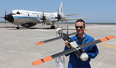
The observations were made by a new type of sUAS, described in a recently published paper in BAMS, called the Coyote that flew below 1 km in hurricanes. Sampling winds, temperature, and humidity in this so-called planetary boundary layer (PBL), the expendable Coyotes flew as low as 136 m in wind speeds as high as 87 m s-1 (196 mph) and for as long as 40 minutes before crashing (as intended) into the ocean.
In the BAMS article, Joe Cione at al. describe the value of and uses for the low-level hurricane observations:
Such high-resolution measurements of winds and thermodynamic properties in strong hurricanes are rare below 2-km altitude and can provide insight into processes that influence hurricane intensity and intensity change. For example, these observations—collected in real time—can be used to quantify air-sea fluxes of latent and sensible heat, and momentum, which have uncertain values but are a key to hurricane maximum intensity and intensification rate.
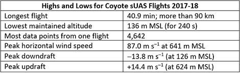
Coyote was first deployed successfully in Hurricane Edouard (2014) from NOAA’s WP-3 Orion hurricane hunter aircraft. Recent Coyote sUAS deployments in Hurricanes Maria (2017) and Michael (2018) include the first direct measurements of turbulence properties at low levels (below 150 m) in a hurricane eyewall. In some instances the data, relayed in near real-time, were noted in National Hurricane Center advisories.
Turbulence processes in the PBL are also important for hurricane structure and intensification. Data collected by the Coyote can be used to evaluate hurricane forecasting tools, such as NOAA’s Hurricane Weather Research and Forecasting (HWRF) system. sUAS platforms offer a unique opportunity to collect additional measurements within hurricanes that are needed to improve physical PBL parameterization.
Images were captured from a video courtesy of Raytheon Corporation.
The authors write that during some flights instrument challenges occurred. For example:
thermodynamic data were unusable for roughly half of the missions. Because the aircraft are not recovered following each flight, the causes of these issues are unknown. New, improved instrument packages will include a multi-hole turbulence probe, improved thermodynamic and infrared sensors, and a laser or radar altimeter system to provide information on ocean waves and to more accurately measure the aircraft altitude.
Future uses of the sUAS could include targeting hurricane regions for observations where direct measurements are rare and models produce large uncertainty. Meanwhile, the article concludes, efforts are underway to increase sUAS payload capacity, battery life, and transmission range so that the NOAA P-3 need not loiter nearby.
"Megaflashes": How Long Can a Lightning Discharge Be?
Even though Earth’s atmosphere is laced by more than a billion brilliant discharges of electricity every year, lightning itself never seems ordinary. But there’s a broad range of lightning, and sometimes, at the extreme, it’s possible to recognize a difference between the ordinary and amazing, even among lightning flashes. The challenge is finding and observing such extremes.
New research by Walt Lyons and colleagues, published in BAMS, reports such a perspective-altering observation of long lightning flashes. To appreciate the observation, consider first the “ordinary” lightning flash. The charge center of the cloud itself is typically 6–10 km above ground. And from there the lightning doesn’t necessarily go straight down: it may extend horizontally, even 100 km or more. Typical lightning might be best measured in kilometers or a few tens of kilometers.
A world record flash in 2007 meandered across Oklahoma for “approximately 300 km.” But that may be a mere cross-counties commute compared to newly discovered interstate “megaflashes” that are almost twice as long. One such megaflash, as the BAMS paper names them, sparked across the sky for ~550 km from northeast Texas across Oklahoma to southeast Kansas in October 2017. And this megaflash, too, may not be the longest ̶ it just happened to occur within the Oklahoma lightning mapping array (OK LMA), allowing for its full study.
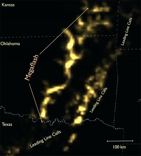
Also, just like the official record flash, which produced 13 cloud-to-ground (CG) lightning strikes, including two triggering sprites that shot high into the atmosphere, this horizontal megaflash also triggered a plethora of CG bolts, in-cloud discharges, and upward illuminations during its 7.18 second lifespan.
The new Geostationary Lightning Mapper sensor on the GOES-16/17 satellite has become the latest tool suited to investigating long-path lightning. The BAMS paper says the sensor is showing that a megaflash “appears able to propagate almost indefinitely as long as adequate contiguous charge reservoirs exist” in the clouds. Such conditions seem to be present in mesoscale convective systems—large conglomerates of thunderstorms that extend rainy stratiform clouds across many hundreds of km. The paper adds,
Megaflashes also pose a safety hazard, as they can be thought of as the stratiform region’s version of the ‘bolt-from-the blue,’ sometimes occurring long after the local lightning threat appears to have ended. But some key questions remain – what is the population of megaflashes and how long can they actually become?
The authors conclude:
Is it possible that a future megaflash can attain a length of 1000 km? We would not bet against that. Let the search begin.
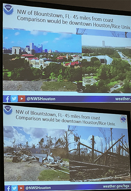
What If: Hurricane Michael's Extensive Wind Swath Would Devastate Houston, NWS says
“In summary, it’s going to be bad.”
That’s how Jeff Evans with the NWS in Houston/Galveston began Wednesday’s presentation, “What if Hurricane Michael Struck Houston? An Examination of Inland Wind Damage,” at the AMS 100th Annual Meeting in Boston.
He was boots on the ground after Hurricane Michael slammed the panhandle as a Category 5 with 160 mph winds on October 10, 2018, assisting the Tallahassee NWS office with surveying the widespread wind damage that extended well away from the coast. Because Michael was intensifying at landfall as well as accelerating, its extreme winds spread deep inland, across the panhandle and well into southwest and southern Georgia.
The Donalsonville, Georgia, airport northeast of Marianna, Florida, and about 90 miles inland, recorded a wind gust to 115 mph, while Marianna had a gust to 103 mph in Michael. Both as well as Blountstown, Georgia, suffered significant damage to structures as well as trees.
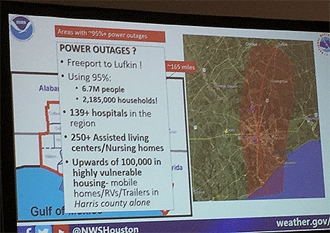
Evans overlaid maps of Michael’s track, wind swath, and areal power outages on Houston to show the extent of its damage potential. The entire Houston metro area with 7.1 million people would suffer; 6.9 million would lose power. And damage to homes and devastation to the landscape would mimic the widespread destruction he observed in the Florida panhandle and southern Georgia where entire forests were virtually flattened.
Evans said that as an NWS meteorologist responsible for warning the Houston area if such a scenario threatened he would have a lot of trouble following the standard hurricane mantra, “Run from the water, hide from the wind.”
“Telling people inland to stay put in such extreme wind conditions is not something I would want to do,” he says.
But, he adds, telling them to get out could prove just as deadly in the mass exodus.
“When you start talking about storms, such as Rita, with 130 mph winds or higher, it’s a spontaneous evacuation.” More than 50 people died just from the evacuation of Houston ahead of that storm, he says
It’s been 37 years since a storm brought a significant wind threat to the Houston area. Hurricane Alicia in 1983 was the last. Hurricane Harvey in 2017 was a widespread catastrophic flood event. Hurricane Ike in 2008 was primarily a surge storm.
“The population in and around Houston has doubled during that time,” Evans says. A 2015 American Community Survey showed more than 130,000 people in just Harris county who live in mobile homes, with thousands more in the surrounding counties.
He conducted the research to raise awareness of a “Michael-like” storm and the immense challenges it would represent.